Displace images with a linear and homogeneous deformation function

In this example a linear homogeneous deformation function \(\Phi\) is firstly created and then is used to deform an image.

Import modules

import matplotlib.pyplot as plt
import spam.deformation
import spam.DIC
import spam.datasets

Load and show data

snow = spam.datasets.loadSnow()

print(snow.shape)

# Show the middle horizontal slice of the snow data set, visualised with ``matplotlib``
plt.figure()
plt.title("Horizontal slice through original dataset")
plt.imshow(snow[50], cmap='Greys_r', vmin=8000, vmax=36000)

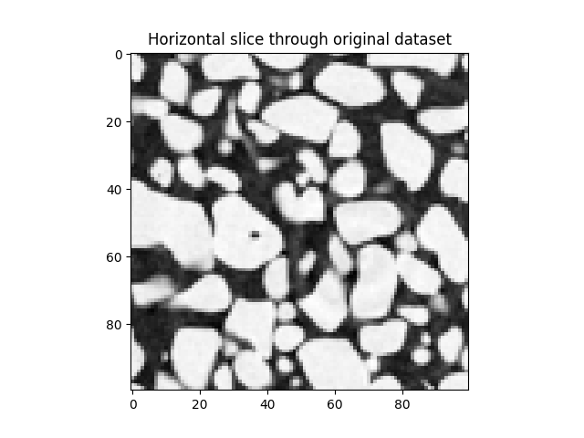
(100, 100, 100)

<matplotlib.image.AxesImage object at 0x7f15b0b11290>

Apply a displacement

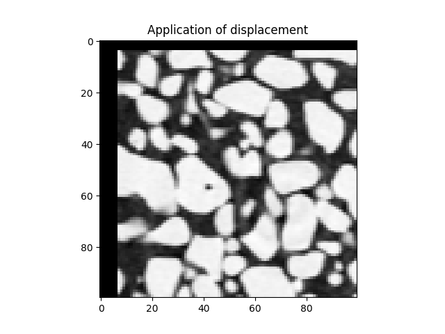
Let’s build a \(\Phi\) corresponding to an in-plane (i.e., X and Y) translation of 3 pixels in the Y direction and 5.5 pixels in the X direction (although given that it is a pure translation it would be pretty easy to manually write all the components of \(\Phi\) by hand).

Please note: Since trilinear image interpolation is enabled by default, applying a displacement of 5.5 in the X direction is indeed meaningful.

transformation = {'t': [0.0, 3.0, 5.5]}

Phi = spam.deformation.computePhi(transformation)

# Apply :math:`\Phi` to the snow volume
snowDeformed = spam.DIC.applyPhi(snow, Phi=Phi)

# The output will still be 100x100x100, meaning that some data's been lost.
print(snowDeformed.shape)
# output: (100, 100, 100)

# Show the middle horizontal slice of the deformed snow data set
plt.figure()
plt.title("Application of displacement")
plt.imshow(snowDeformed[50], cmap='Greys_r', vmin=8000, vmax=36000)

(100, 100, 100)

<matplotlib.image.AxesImage object at 0x7f15dfe9ee90>

Apply a rotation

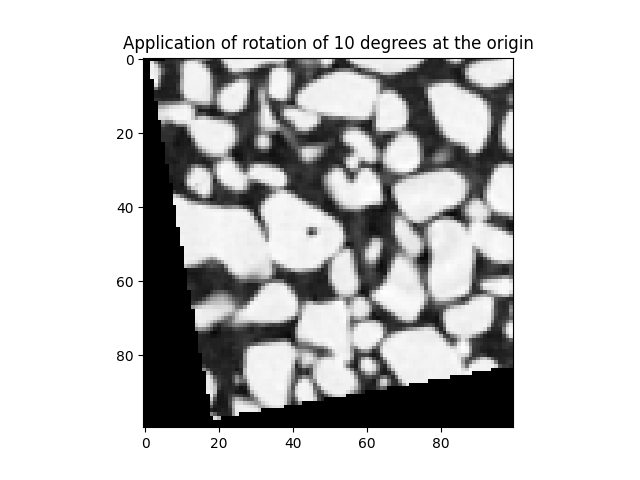
Mathematically speaking, rotations are applied around the origin:

$$O = (0,0,0)$$

Which in this case is not the middle of the image, but the top-left-back of the image, which is a little unnatural for the application of rotations. Let’s apply a +10 degree rotation (i.e., anti-clockwise) and overwrite our translation and \(\Phi\) and check:

transformation = {'r': [10.0, 0.0, 0.0]}
Phi = spam.deformation.computePhi(transformation)
print(Phi)

[[ 1.     0.     0.     0.   ]
 [ 0.     0.985 -0.174  0.   ]
 [ 0.     0.174  0.985  0.   ]
 [ 0.     0.     0.     1.   ]]

There are no translations (0,0,0,1 in the right-most column), so this is a pure rotation. Mathematically speaking, rotations are defined as positive-anticlockiwse around the origin at (0,0,0). Let’s apply it to the snow dataset in the same way as above :

snowDeformed = spam.DIC.applyPhi(snow, Phi=Phi, PhiCentre=[0.0, 0, 0.0])

# Show the middle horizontal slice of the deformed snow data set
plt.figure()
plt.title("Application of rotation of 10 degrees at the origin")
plt.imshow(snowDeformed[50], cmap='Greys_r', vmin=8000, vmax=36000)

<matplotlib.image.AxesImage object at 0x7f15b0d34f10>

It is usually more logical to apply \(\Phi\) (if it is anything other than a pure translation) to the middle of the image – this is the default behaviour (i.e., PhiPoint = (numpy.array(im.shape) - 1) / 2.0)):

snowDeformed = spam.DIC.applyPhi(snow, Phi=Phi)

# Show the middle horizontal slice of the deformed snow data set
plt.figure()
plt.title("Application of rotation of 10 degrees at 50,50,50 (centre)")
plt.imshow(snowDeformed[50], cmap='Greys_r', vmin=8000, vmax=36000)
plt.show()

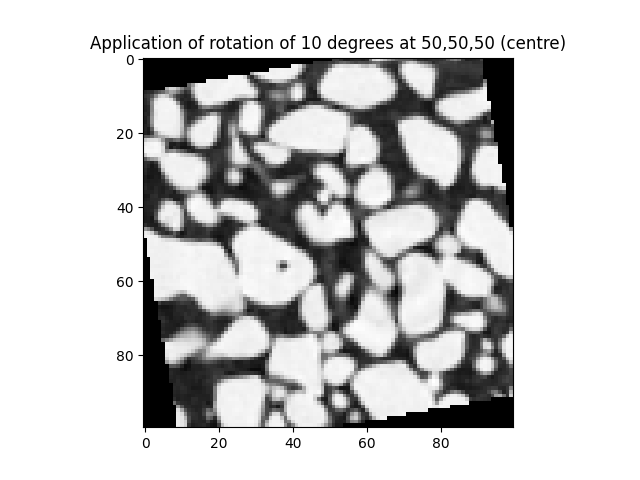
You can see that the point of application of this linear transformation is important.