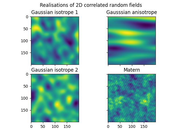
Simulation of correlated Random Fields

Example of a generation of 2D correlated Random Field

from spam.excursions import simulateRandomField
import matplotlib.pyplot as plt

# generate two gaussian isotrope
covarianceParameters = {"len_scale": 0.1}
r1 = simulateRandomField(nNodes=200, covarianceModel="Gaussian", covarianceParameters=covarianceParameters, dim=2, nRea=2)

# generate one gaussian anisotrope
covarianceParameters = {"len_scale": [0.1, 0.5]}
r2 = simulateRandomField(nNodes=200, covarianceModel="Gaussian", covarianceParameters=covarianceParameters, dim=2, nRea=2)

# generate one matern
covarianceParameters = {"len_scale": 0.1, "nu": 0.4}
r3 = simulateRandomField(nNodes=200, covarianceModel="Matern", covarianceParameters=covarianceParameters, dim=2)

# plot
fig = plt.figure()
fig.suptitle("Realisations of 2D correlated random fields")
gs = fig.add_gridspec(2, 2)
axes = gs.subplots()
axes[0, 0].imshow(r1[0])
axes[0, 0].set_title("Gaussian isotrope 1")
axes[1, 0].imshow(r1[1])
axes[1, 0].set_title("Gaussian isotrope 2")
axes[0, 1].imshow(r2[0])
axes[0, 1].set_title("Gausssian anisotrope")
axes[1, 1].imshow(r3[0])
axes[1, 1].set_title("Matern")

for ax in fig.get_axes():
    ax.label_outer()

plt.show()