
Tutorial: Image correlation – Practice#
This is not a general tutorial for doing image correlation. As explained in Scripts in spam, we provide different image correlation scripts, depending on the imaged texture and the deformation between the two imaged states.
You’re in the right place:
If you’re coming from Tutorial: Image correlation – Theory, and your objective is to get a first practical introduction with the deformation function, Φ, used in spam
If you want to measure a deformation field defined at a grid of regularly-spaced points – see also Regular grid local DIC script (spam-ldic).
Note
If you have discrete particles and you want to do particle tracking, read the initial guess part of the tutorial, and then go here: Tutorial: Discrete Image correlation.
Manipulating Φ#
As seen in the theory part, although very powerful, Φ matrices can be hard to handle compared to separated components of translation, rotation, etc.
For this reason, spam provides a number of helper functions inside spam.deformation module. For example you can create your own deformation function Φ like this:
# (This is in iPython)
import spam.deformation

# Create a "transformation" dictionary containing a rotation "R" of 15°
# around the z-axis and a translation "t" of z=3, y=1.3, x=2.2 px
transformationIn = {'t': [3.0, 1.3, 2.2], 'r': [15.0, 0.0, 0.0]}
# The other options are "z" for zoom and "s" for shear

Phi = spam.deformation.computePhi(transformationIn)

print(Phi)
# output:
#   [[ 1.     0.     0.     3.   ]
#    [ 0.     0.966 -0.259  1.3  ]
#    [ 0.     0.259  0.966  2.2  ]
#    [ 0.     0.     0.     1.   ]]
The input translation vector in the fourth column of the matrix, while the remaining components of the deformation are mixed inside the 3x3 top-left sub-matrix.
We offer a function to separate these components into an object which resembles the transformation dictionary used in the example above. Note that the decomposition of the top left 3x3 matrix in Φ is based on the polar decomposition explained in detail in Tutorial: Refreshments in continuum mechanics.
# (Following from example above)
transformationOut = spam.deformation.decomposePhi(Phi)

for key in transformationOut.keys():
    print(key, transformationOut[key])

# output (order here not guaranteed):
#
#   t
#       [3., 1.3, 2.2]
#
#   r
#       [15., 0., 0.]
#
#   z
#       [1.0, 1.0, 1.0]
#
#   vol
#       -1.1102230246251565e-16
#
#   dev
#       0.0
#
#   U
#       [[1. 0. 0.]
#        [0. 1. 0.]
#        [0. 0. 1.]]
#
#   volss
#       -0.06814834742186338
#
#   devss
#        0.02782144633291313
#
#   e
#        [[ 0.     0.     0.   ]
#         [ 0.    -0.034  0.   ]
#         [ 0.     0.    -0.034]]
#
Both the rotation “r” and the translation “t” are obtained back from the decomposed Φ.
The 3x3 U matrix corresponds to the right stretch tensor, as explained in Tutorial: Refreshments in continuum mechanics. It is equal to the identity matrix, since rotations and translations are only a rigid-body motion and no strains are involved.
The “z” or zoom component (for consistency with scipy.ndimage.zoom) corresponds to the diagonal components of the above stretch tensor U and shows here that there is no change of size of the image.
Thereafter, there are strain invariants under the framework of large strains (see details in Tutorial: Strain calculation). The volumetric strain – “vol” – and the deviatoric strain – “dev” –, which are both zero, as you can see.
Strains under the framework of small (infinitesimal) stains theory are also shown (see details in Tutorial: Strain calculation). “e” stands for ε is the infinitesimal strain tensor, which as you can see in not the identity matrix. Again the two invariants, – “volss” – and – “devss” – which unfortunately are not zero because the small strains framework does not take into account rotations.
Applying a single Φ to an image#
An image can be homogeneously deformed by a single Φ using the function spam.DIC.applyPhi().
It’s important to note that the default centre of application (for example the centre of rotation) is the middle of the image.
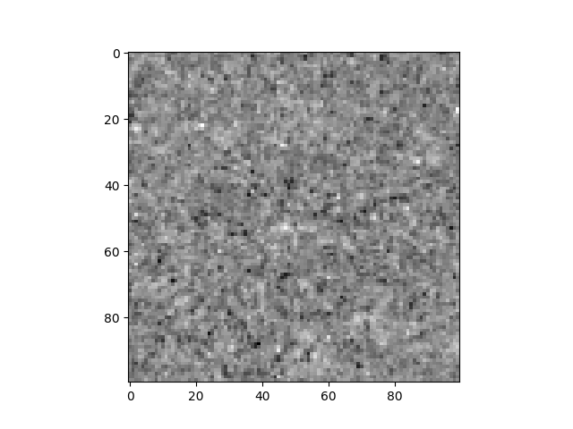
Here we will use the snow dataset, which is a small 100x100x100 crop out of a reconstructed x-ray attenuation field of snow grains performed at 15 μm/px. This small volume is one of the proposed datasets in spam, and you can find it inside tools/data/snow. Here is a simple 3D rendering:
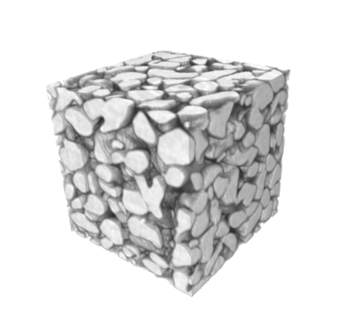
Data Credits: from an experiment by Peinke et al. from CEN / CNRM / Météo-France - CNRS and scanned in the Laboratoire 3SR micro-tomograph#
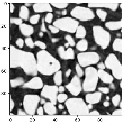
A slice through the 3D volume above#
For a better insight into the deformation function Φ, but also to understand the importance of the centre of application of Φ, please have a look at the example here: Displace images with a linear and homogeneous deformation function.
The remaining of this tutorial is dedicated to the measurement of a field of deformation functions that map two images.
Before starting the correlation#
Measuring a field of Φs between two images can be slow and error-prone. Thus, before launching an image correlation script, it’s important to clarify a certain number of points.
The use of image binning#
The appearance of the gradient term introduced in the previous tutorial is a clear sign that what is needed for a good correlation is edges.
One excellent strategy to make image correlation more robust and faster is to use binning. This means averaging voxels together in space, meaning that the 100x100x100 image used above will become 50x50x50 with binning 2.
In spam, there is a function called spam.DIC.binning() that handles the downscaling of the images. This has three advantages:
Spatial averaging reduces the measurement noise in the measured deformation
High-frequency content i.e., small spatial variations are erased, which will help the coarse gradients to converge
An 8-times smaller 3D image will correlate much faster
The amount of binning that can be done to a given image depends on the coarsest texture – if it is erased by binning then that is too much binning.
An objective measurement of this is the correlation length that comes from the spam.measurements toolkit.
Please see also the example here: Compute covariance.
Initial guess#
Remember that the iterative algorithm implemented in spam.DIC.register() (described in the previous tutorial) will only converge if we’re close to the right solution.
Fortunately, there’re certain steps that can bring us closer to this solution, and in spam these steps are implemented as stand-alone scripts. If you haven’t done it so far, please consult the general flowchart for how we recommend to use these different image correlation scripts here Scripts in spam.
If we can summarise this flowchart again quickly, the following options are envisaged:
Practically nothing is happening between the two images, so just directly run
spam.DIC.register()on a set of points defined:
either at a regular grid, see Regular grid local DIC script (spam-ldic), and the remaining of this tutorial
or, the centres of mass of particles, see Tutorial: Discrete Image correlation
There is a homogeneous transformation, described by a single Φ, that roughly maps im1 into im2. You should first measure this Φ (see Registration script (spam-reg)) and then give it as an initial guess to your set of points.
There is a complex transformation mapping im1 into im2 and a single Φ does not get you close enough. In this case the script Pixel search script (spam-pixelSearch) is needed: a coarse nearest-pixel displacement-only raster scan – not elegant but it is necessary sometimes.
Note
If you have discrete particles and you want to do particle tracking, please continue here: Tutorial: Discrete Image correlation.
Let’s measure a Φ field with spam-ldic#
It is now time to measure a deformation field between two images defined at a set of regularly spaced points. We will create a grid of points in the reference image and try to match small subvolumes centred on each point in order to see how each subvolume deforms.
In our example we’ll use the VEC4 data set – an x-ray tomography of a sandstone performed before and after straining done by E. Charalampidou and used as an example in TomoWarp 2 [TUD2017a]. Please download VEC4.zip from spam tutorial archive on zenodo.
Here is a horizontal slice before and after straining:
import matplotlib.pyplot as plt
import tifffile

VEC4one = tifffile.imread("VEC4-01-b1.tif")
VEC4two = tifffile.imread("VEC4-02-b1.tif")

print(VEC4one.shape)
# output:
#  (760, 551, 551)

plt.figure()
plt.subplot(1,3,1)
plt.imshow( VEC4one[VEC4one.shape[0]//2], cmap="Greys_r" )
plt.subplot(1,3,2)
plt.imshow( VEC4two[VEC4two.shape[0]//2], cmap="Greys_r" )
plt.subplot(1,3,3)
plt.hist( VEC4one.ravel(), bins=256 ); plt.xlabel("Greylevel"); plt.ylabel("Count")
plt.show()
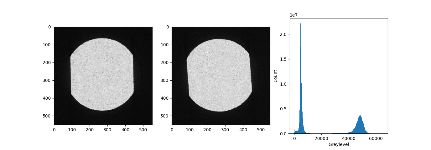
Middle slices from VEC4 dataset scan before and after compression#
So there is clearly a rotation between the before and after image (it’s not that easy to place a sample back exactly). This seems like a good example for #2 of the initial guess discussed above, since a rigid-body rotation can be easily described by a single deformation function.
Step 1: Start by binning the two images#
Before we choose how much we can scale down this image with binning let’s have a look at the texture closely:
# following from above
plt.imshow( VEC4one[VEC4one.shape[0]//2,\
            VEC4one.shape[1]//2-100:VEC4one.shape[1]//2+100,\
            VEC4one.shape[2]//2-100:VEC4one.shape[2]//2+100], cmap="Greys_r")
plt.show()
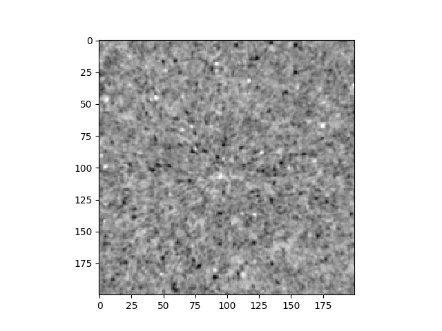
Zoom into 200x200 of the slice#
Let’s now make a binning 2 version of VEC4one by averaging 2×2×2 pixels together using spam’s binning function and show it:
# following from above
import spam.DIC

VEC4oneb2 = spam.DIC.binning(VEC4one, 2)
VEC4twob2 = spam.DIC.binning(VEC4two, 2)

print(VEC4oneb2.shape)
# output:
#  (380, 275, 275)

plt.imshow( VEC4oneb2[VEC4oneb2.shape[0]//2,\
            VEC4oneb2.shape[1]//2-50:VEC4oneb2.shape[1]//2+50,\
            VEC4oneb2.shape[2]//2-50:VEC4oneb2.shape[2]//2+50], cmap="Greys_r")
plt.show()
Zoom into 100x100 of the binning 2 version of the slice above#
Step 2: Run an initial registration#
Some of the coarser texture is preserved, let’s try to measure the rigid-body rotation. There are a number of options for the spam-reg script, which are list if it is called with - -help. Please see: Registration script (spam-reg) for more information on the script. For our example, to show-off, we’ll perform the binning of the two images directly inside the script.
(spam) $ spam-reg \                         # the script
            VEC4-01-b1.tif VEC4-02-b1.tif \ # the two 3D images (tiff files) to correlate
            -bb 2 \                         # ask to start from half-sized images
            -m 40 -g                        # set a 40px margin at each direction, activate graphical mode to look at slices during iterations

            # output:
            #spam-reg -- Current Settings:
            #BIN_BEGIN: 2
            #BIN_END: 1
            #DEF: False
            #GRAPH: True
            #INTERPOLATION_ORDER: 1
            #MARGIN: 40.0
            #MASK1: None
            #MAX_ITERATIONS: 50
            #MIN_DELTA_PHI: 0.0001
            #OUT_DIR: VEC4-bin1
            #PHIFILE: None
            #PHIFILE_BIN_RATIO: 1.0
            #PREFIX: VEC4-01-b1-VEC4-02-b1-registration
            #RIGID: False
            #UPDATE_GRADIENT: False
            #im1: <_io.TextIOWrapper name='VEC4-bin1/VEC4-01-b1.tif' mode='r' encoding='UTF-8'>
            #im2: <_io.TextIOWrapper name='VEC4-bin1/VEC4-02-b1.tif' mode='r' encoding='UTF-8'>

            #spam.DIC.registerMultiscale(): working on binning:  2
            #Start correlation with Error = 1132.80
            #Iteration Number:16   dPhiNorm=0.00007   error=92.93   t=[-0.007 2.044 -1.303]   r=[3.038 -0.488 0.020]   z=[0.994 1.001 1.003] (Elapsed Time: 0:00:25)
            #    -> Converged

            #spam.DIC.registerMultiscale(): working on binning:  1
            #Start correlation with Error = 85.31
            #Iteration Number:7   dPhiNorm=0.00005   error=84.70   t=[-0.031 4.034 -2.552]   r=[3.038 -0.485 0.022]   z=[0.993 1.001 1.003] (Elapsed Time: 0:01:15)
            #    -> Converged

            #Registration converged, great... saving
Please note that the script above saved by default a “.tsv” file with the result of the measured Φ. The registration is successful, getting below the desired deltaPhiNorm of 0.0001. The advantage of using the multiscale approach is clear, since the majority of the measured transformation is accounted for in the half-sized images after 16 iterations. By using this deformation function as an initial condition to the original scale, only 7 iterations were needed.
The registration step appears to be a good initial guess of the deformation of the sample.
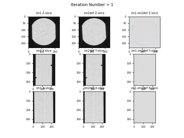
Orthogonal slices and their difference (last coloumn) of VEC4 data after 1 iteration in binning 2 (half-sized images)#
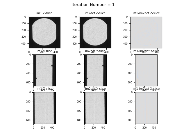
Orthogonal slices and their difference (last coloumn) of VEC4 data after 1 iteration in binning 1 (original size images)#
Step 3: Run spam-ldic script#
It’s now time to run our local correlation script, using as an initial guess the registration result from above. As for spam-reg, there are a number of options for the spam-ldic script, which are list if it is called with - -help. Please see: Regular grid local DIC script (spam-ldic) for more information on the script.
In order to run spam-ldic you need to define a regular grid of points. You can see A note on the correlation grid for tips regarding the grid geometry. In our example, we’ll set the half-window size equal to 10 pixels, a choice made based on the texture. The spacing of the measurement points is set double of the half-window size, so as not to have overlapping correlation windows.
In order to avoid correlating windows that fall into the background, a grey level threshold is set equal to 20000 (see historgram above). An equivalent way to avoid correlating the background is to create a mask of the im1 (reference image), and pass it into the script with the -mf1 argument.
(spam) $ spam-ldic \                                      # the script
            VEC4-01-b1.tif VEC4-02-b1.tif \               # the two 3D images (tiff files) to correlate
            -pf VEC4-01-b1-VEC4-02-b1-registration.tsv \  # the tsv file containing the registration guess
            -hws 10 -ns 20 \                              # half-window size of the correlation window and node spacing (both in pixels)
            -it 10 \                                      # the number of maximum iterations
            -glt 20000 \                                  # do not correlate windows with mean grey level below this (see historgram above)
            -vtk -tif                                     # ask for tif and vtk output files


    # output:
    #spam-ldic -- Current Settings:
    #APPLY_F: all
    #GREY_HIGH_THRESH: inf
    #GREY_LOW_THRESH: 20000.0
    #HWS: [10, 10, 10]
    #INTERPOLATION_ORDER: 1
    #MARGIN: [3, 3, 3]
    #MASK1: None
    #MASK_COVERAGE: 0.5
    #MAX_ITERATIONS: 10
    #MIN_DELTA_PHI: 0.001
    #NS: [20, 20, 20]
    #OUT_DIR: VEC4-bin1
    #PHIFILE: <_io.TextIOWrapper name='VEC4-bin1/VEC4-01-b1-VEC4-02-b1-registration.tsv' mode='r' encoding='UTF-8'>
    #PHIFILE_BIN_RATIO: 1.0
    #PREFIX: None
    #PROCESSES: 8
    #SERIES_INCREMENTAL: False
    #TIFF: True
    #TSV: True
    #UPDATE_GRADIENT: False
    #VTK: True
    #inFiles: [<_io.TextIOWrapper name='VEC4-bin1/VEC4-01-b1.tif' mode='r' encoding='UTF-8'>, <_io.TextIOWrapper name='VEC4-bin1/VEC4-02-b1.tif' mode='r' encoding='UTF-8'>]

    #Correlating: VEC4-01-b1-VEC4-02-b1
    #I read a registration from a file in binning 1.0
    #Translations (px)
    #    [-0.031  4.034 -2.552]
    #Rotations (deg)
    #    [ 3.038 -0.485  0.022]
    #Zoom
    #    [0.9934788644484028, 1.0010511380127196, 1.0033909227620816]

    #Starting local dic (with 8 processes)
        #it=005  dPhiNorm=0.0003  rs=+2  |###################################################| Time: 0:00:32
Let’s go and see what’s in output:
bash> ls -l output/
total 8096
-rw-rw-r-- 1 ostamati ostamati  114620 sept. 30 17:24 VEC4-01-b1-VEC4-02-b1-ldic-deltaPhiNorm.tif
-rw-rw-r-- 1 ostamati ostamati  114620 sept. 30 17:24 VEC4-01-b1-VEC4-02-b1-ldic-error.tif
-rw-rw-r-- 1 ostamati ostamati  114620 sept. 30 17:24 VEC4-01-b1-VEC4-02-b1-ldic-iterations.tif
-rw-rw-r-- 1 ostamati ostamati  114620 sept. 30 17:24 VEC4-01-b1-VEC4-02-b1-ldic-returnStatus.tif
-rw-rw-r-- 1 ostamati ostamati 5265438 sept. 30 17:24 VEC4-01-b1-VEC4-02-b1-ldic.tsv
-rw-rw-r-- 1 ostamati ostamati 2217738 sept. 30 17:24 VEC4-01-b1-VEC4-02-b1-ldic.vtk
-rw-rw-r-- 1 ostamati ostamati  114620 sept. 30 17:24 VEC4-01-b1-VEC4-02-b1-ldic-Xdisp.tif
-rw-rw-r-- 1 ostamati ostamati  114620 sept. 30 17:24 VEC4-01-b1-VEC4-02-b1-ldic-Ydisp.tif
-rw-rw-r-- 1 ostamati ostamati  114620 sept. 30 17:24 VEC4-01-b1-VEC4-02-b1-ldic-Zdisp.tif
Here you can see big TSV and VTK files, which contain all the correlation information for all points. You can also see a number of other TIFF files, which contain 3D fields encoding the results of the correlation, and a number of “disp” TIFF files which show the displacement field (extracted from each local Φ). Let’s look at the returnStatus file – here we will load it in Fiji and look at a vertical slice:

Central vertical slice through returnStatus, white = 2 (Converged), grey = 1 (Stopped on number of iterations), black = -5 (Did not correlate due to too-low greyscale value –based on given -glt)#
The fact that there are some points that have been stopped with the maximum number of iterations 10 is a pity. Let’s relaunch the calculation with more iterations, without the line -it 10 to the command line above. Now the default number of iterations (which is set to 50) is considered, so we rerun the spam-ldic script above with -ii 50, which practically doesn’t increase the computation time since few points require more iterations.

As above but with 50 iterations rather than 10. Vertical slice through returnStatus, white = 2 (Converged), grey = 1 (Stopped on number of iterations), black = -5 (Did not correlate due to too-low greyscale value –based on given -glt)#
That’s better. Let’s have a look at the displacement field. Let’s load “Zdisp.tif”:
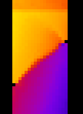
Central vertical slice through Z (vertical) displacement field shown with the “fire” LUT. Values shown are from -4 +4 pixels, and reveal a very clear zone of localised strain.#
To see this as a “full” displacement field, the VTK file can be dragged and dropped into ParaView (then activate Glyph mode and threshold on returnStatus = 2).
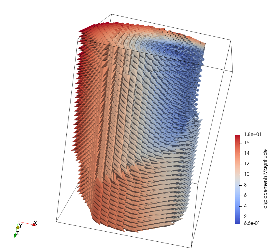
The resulting displacement field (including the rigid-body motion – Z rotation)#
Computing strains from the displacement field#
Now that we’ve measured a displacement field on a regular grid, please head over to the Tutorial: Strain calculation for a complete description of the calculation of strain.