Expectation of global descriptors in 1D

This example shows how to compute theoretical expectations of total length (L1) and Euler characteristic (L0) of excursion sets as a function of the excursion’s threshold. Excrusions are define here as the subdomain of the domain where the Random Field is defined where the Random Field values are above a certain threshold.

Here the two measures are seen as function of the threshold value.

Monte Carlo results are confronted to the theory.

import spam.excursions
import spam.measurements
import matplotlib.pyplot as plt
import numpy

Correlated Random Field parameters

First we set all the correlated Random Fields parameters. It is assumed that the distribution is Gaussian with zero mean and the covariance function is Gaussian too.

# set the variance
variance = 1.0
# standard deviation
std = numpy.sqrt(variance)
# correlation length
correlationLength = 10
# length of the domain
length = 100.0

# set the thresholds between -5 and 5
thresholds = numpy.linspace(-5, 5, 50)

Compute the two theoretical expected measures

The two measures of the excursion (total length (1) and Euler characteristic (0)) are computed and ploted for every thresholds

# spatial dimension
spatialDimension = 1
# the measure number 1
totalLength = spam.excursions.expectedMesures(thresholds, 1, spatialDimension, std=std, lc=correlationLength, a=length)
# the measure number 0
eulerCharac = spam.excursions.expectedMesures(thresholds, 0, spatialDimension, std=std, lc=correlationLength, a=length)

# plt.figure()
# plt.xlabel("Threshold")
# plt.title("Total length")
# plt.plot(thresholds, totalLength, 'r')
#
# plt.figure()
# plt.xlabel("Threshold")
# plt.title("Euler characteristic")
# plt.plot(thresholds, eulerCharac, 'r')

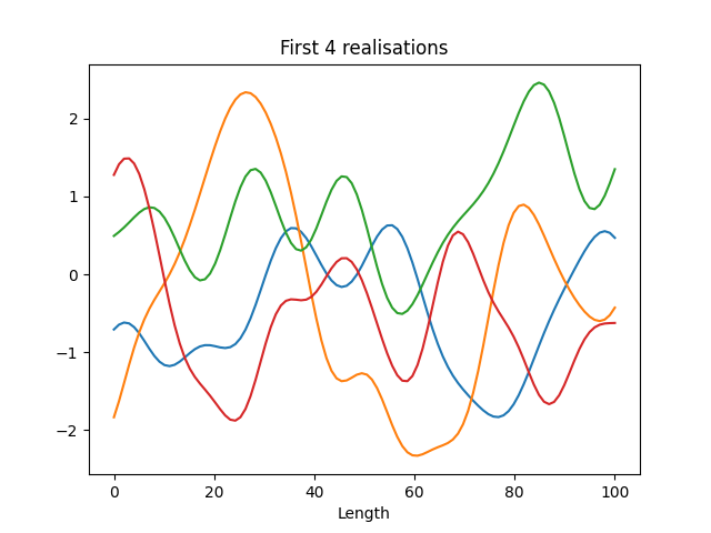
Generate 1000 realisations of the correlated Random Field

In order to compare the theoretical values to Monte Carlo results, first 1000 realisations of a correlated Random Field are generated.

# number of realisations
nRea = 500
nNodes = 100

# define the covariance
covarianceParameters = {'len_scale': correlationLength, 'var': variance}

# generate realisations
realisations = spam.excursions.simulateRandomField(lengths=length, nNodes=nNodes, covarianceParameters=covarianceParameters, dim=spatialDimension, nRea=nRea)

plt.figure()
plt.xlabel("Length")
plt.title("First 4 realisations")
for i in range(4):
    plt.plot(numpy.linspace(0, length, nNodes), realisations[i])

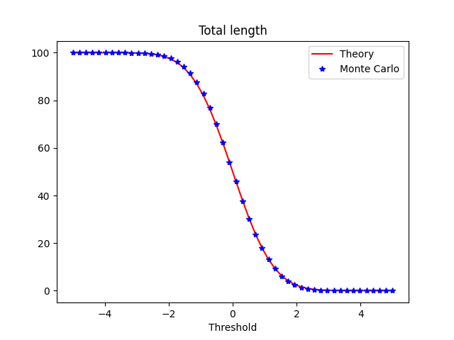
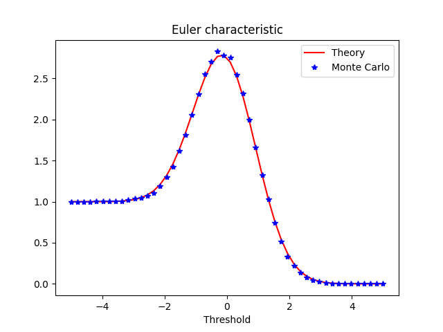
Compute the two averaged measures

For every thresholds, the two average measures over all the realisations are compute and compared to the theoretical values.

# save average for every thresholds
totalLengthMC = numpy.zeros_like(thresholds)
eulerCharacMC = numpy.zeros_like(thresholds)
# coucou

# loop over the thresholds
for i, t in enumerate(thresholds):
    # loop over the realisations
    for r in realisations:
        totalLengthMC[i] += length * spam.measurements.volume(r > t) / float(nRea * nNodes)
        eulerCharacMC[i] += spam.measurements.eulerCharacteristic(r > t) / float(nRea)

# plot length
plt.figure()
plt.xlabel('Threshold')
plt.title('Total length')
plt.plot(thresholds, totalLength, 'r', label='Theory')
plt.plot(thresholds, totalLengthMC, '*b', label='Monte Carlo')
plt.legend()

# plot Euler characteristic
plt.figure()
plt.xlabel('Threshold')
plt.title('Euler characteristic')
plt.plot(thresholds, eulerCharac, 'r', label='Theory')
plt.plot(thresholds, eulerCharacMC, '*b', label='Monte Carlo')
plt.legend()
plt.show()

• 
•