Generation of synthetic morphologies based on excursion sets

Exemple of generation of random morphologies based on excrusion sets of correlated Random Fields. The volume and the surface area are targeted and used to set the statistical parameters of the Random Field. Then 2 realisations of such excursions are generated and global descriptors computed.

import spam.excursions
import spam.measurements
import matplotlib.pyplot as plt

Characteristics of the morphologies

We start by setting the parameters of the morphology For example here, we choose to generate morphology in 3 dimensions with a volume of 0.2 and a surface area of 5

spatialDimension = 3
targetVolume = 0.2
targetSurface = 5.0
print("Targeted Values")
print("\t volume = {:.2f}".format(targetVolume))
print("\t surface = {:.2f}".format(targetSurface))

Targeted Values
         volume = 0.20
         surface = 5.00

Characteristics Random Field

From the morphological Characteristics retained we can deduce the statistical parameters of the correlated Random Fields and the threshold of the excursion [see https://doi.org/10.1016/j.commatsci.2015.02.039 for details]. For simplicity we choose here to only play on the threshold of the excursion and the correlation length of the Random Field

threshold = spam.excursions.getThresholdFromVolume(targetVolume, 0.0)
correlationLength = spam.excursions.getCorrelationLengthFormArea(targetSurface, 0.1, threshold)
print("Excursion set parameters found")
print("\t threshold = {:.2f}".format(threshold))
print("\t correlation length = {:.2f}".format(correlationLength))

# we can now compute the 4 expected values of the global descriptors of the resulting excurions
volume = spam.excursions.expectedMesures(threshold, 3, spatialDimension, lc=correlationLength)
surface = 2.0 * spam.excursions.expectedMesures(threshold, 2, spatialDimension, lc=correlationLength)
curvature = spam.excursions.expectedMesures(threshold, 1, spatialDimension, lc=correlationLength)
euler = spam.excursions.expectedMesures(threshold, 0, spatialDimension, lc=correlationLength)
print("Expected Values")
print("\t volume = {:.2f}".format(volume))
print("\t surface = {:.2f}".format(surface))
print("\t curvature = {:.2f}".format(curvature))
print("\t euler = {:.0f}".format(euler))

Excursion set parameters found
         threshold = 0.84
         correlation length = 0.17
Expected Values
         volume = 0.20
         surface = 5.00
         curvature = 10.50
         euler = 8

Generation of the morphologies

We can now generate the morphologies. 2 realisations are made here.

# define the covariance with the statistical parameters of the correlated random field
covarianceParameters = {'len_scale': correlationLength}
# generate the random field realisations
nRea = 1  # create 2 realisations
nNodes = 100  # number of node / edge for the random field discretisation
realisations = spam.excursions.simulateRandomField(nNodes=nNodes, covarianceParameters=covarianceParameters, nRea=nRea, dim=spatialDimension, vtkFile="spamPaper")
# realisation is a list of (100, 100, 100) numpy array containing the 2 realisations of the correlated random field

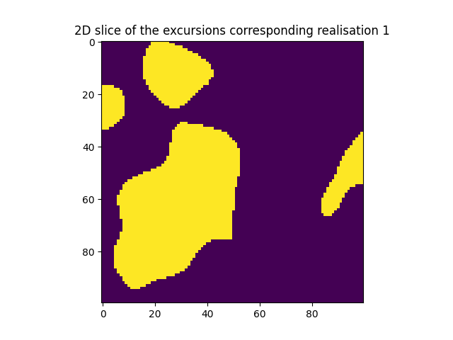
# create the excursions from the random field realisations
excursions = realisations > threshold

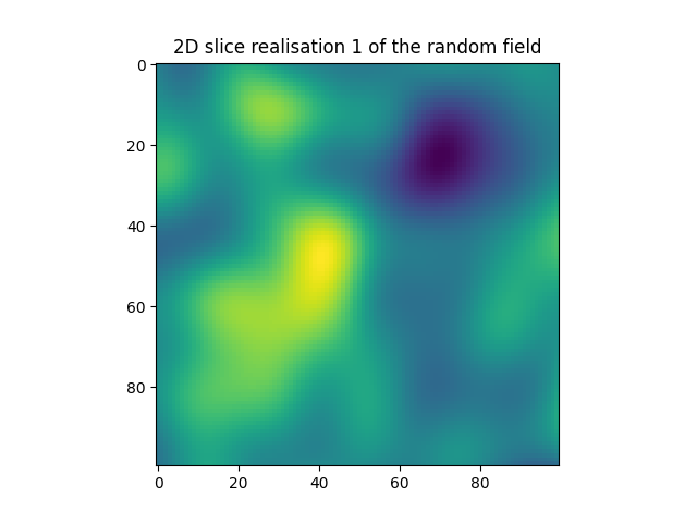
# plot both random field and excursion
for i in range(nRea):
    plt.figure()
    plt.imshow(realisations[i][int(nNodes / 2), :, :])
    plt.title("2D slice realisation {} of the random field".format(i + 1))
    plt.figure()
    plt.imshow(excursions[i][int(nNodes / 2), :, :])
    plt.title("2D slice of the excursions corresponding realisation {}".format(i + 1))

• 
• 

Generating spamPaper_0000... 4.48 seconds

Compute the actual global measures

We can now compute the actual global descriptors of the morphologies to compare them to the theoretical expectations. It can be noted that due to the different aspect of each measure, both volume and Euler characteristic need a boolean array corresponding to the excursion where surface area and total mean curvature need a continuous field and a threshold (level).

for i in range(nRea):
    rea = realisations[i][:, :, :]
    exc = excursions[i][:, :, :]
    aspectRatio = [1. / float(nNodes - 1), 1. / float(nNodes - 1), 1. / float(nNodes - 1)]
    print("Actual values for realisation number {}".format(i + 1))
    print("\t volume = {:.2f}".format(spam.measurements.volume(exc, aspectRatio=aspectRatio)))
    print("\t surface area = {:.2f}".format(spam.measurements.surfaceArea(rea, level=threshold, aspectRatio=aspectRatio)))
    print("\t total mean curvature = {:.2f}".format(spam.measurements.totalCurvature(rea, level=threshold, aspectRatio=aspectRatio)))
    print("\t Euler characteristic = {}".format(spam.measurements.eulerCharacteristic(exc)))
plt.show()

Actual values for realisation number 1
         volume = 0.20
         surface area = 4.58
         total mean curvature = 26.73
         Euler characteristic = 6