Tutorial: Label Toolkit#

Getting started#

Here we will look at how to use the label toolkit to rapidly create and interface with labelled images. The granual dataset is a series of x-ray tomographies acquired during the triaxial compression of a small sample of a Martian Simulant soil, performed in Laboratoire 3SR, Grenoble. Please download M2EA05.zip from spam tutorial archive on zenodo.

To save time we will perform our analysis in a binning 2 version of M2EA05 data by averaging 2×2×2 pixels together using spam’s binning function. If you’ve followed the previous tutorials, we can load this data set in iPython:

import tifffile
import spam.DIC
import matplotlib.pyplot as plt

grey = spam.DIC.binning(tifffile.imread("M2EA05-01-bin2.tif"), 2) # downscale the image while reading it
# tifffile.imsave("M2EA05-01-bin4.tif", grey) # save it for later

plt.imshow(grey[:, :, grey.shape[2]//2], cmap="Greys_r"); plt.show()

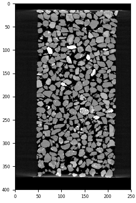
../_images/lab-A-vertSlice.png — A vertical slice through the “Martian Simulant” M2EA05-01-bin4 dataset from [Kawamoto2016]#

Sand grains are clearly visible. Let’s see if we can easily binarise this data by applying a threshold. We can use the internal command for plotting a histogram:

import spam.plotting
spam.plotting.plotGreyLevelHistogram(grey, showGraph=True)

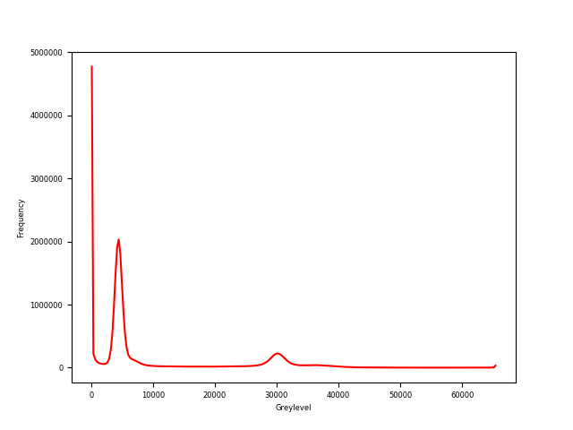
../_images/lab-B-histo.png — Histogram of greylevels of image M2EA05-01-bin4#

Binarisation#

In order to binarise this image we will just take a value between the peaks. Here a lot of refinement is possible, such as measuring against a calibration, or using some histogram-fitting techniques like Otsu’s method. Some techniques are available in skimage.filters Let’s take a threshold of 18000:

# following from above
binary = grey >= 18000 # i.e., binary is where "grey" is bigger than or equal to 18000

print(binary.sum()) # let's count the number of "True" voxels:
# output:
# 4985517

plt.imshow(binary[:, :, binary.shape[2]//2], cmap="Greys_r"); plt.show()

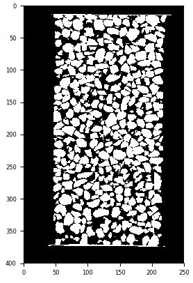
../_images/lab-C-vertSlice-bin.png — Result of applying a greyscale threshold of 18000#

Watershed#

This is clearly “just” a black-and-white image. We need to split these particles up into individually-labelled grains. Let’s use the ITK watershed [ITK2006] to do that through a very simplified interface that we offer:

import spam.label
labelled = spam.label.watershed(binary) # about 3 minutes on Eddy's laptop
# tifffile.imsave(""M2EA05-01-bin4-watershed.tif", labelled) # save it for later

print(labelled.max())
# output:
# 3105
# *i.e.,* there are 3105 different particles

# use spam.label.randomCmap to show different labels
plt.imshow(labelled[:, :, labelled.shape[2]//2], cmap=spam.label.randomCmap); plt.show()

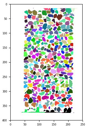
../_images/lab-D-vertSlice-lab.png — Individually labelled particles thanks to ITK’s watershed algorithm. spam.label.randomCmap uses this random colourmap trick. The “glasbey” and “glasbey_inverted” on ImageJ are also good for visualising labels#

Manipulating labelled images#

In such a labelled image, each grain has an individual, integer label, and all of its voxels are replaced by that number. Dealing with such images is what the label toolkit is for. scipy.ndimage has a find_object routine, but ours is much faster. Let’s play – first we will get all the volumes of all the particles:

volumes = spam.label.volumes(labelled)

plt.hist(volumes, bins=64); plt.xlabel("Volume (vx)"); plt.ylabel("count"); plt.show()

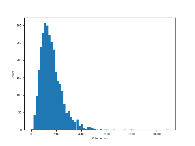
../_images/lab-E-particleVolumeDist.png — Particle volume distribution of particles in M2EA05-01-bin4#

That’s interesting. We can see that the volumes call has actually also asked for bounding boxes of all particles to be calculated. Let’s have a look at what that means:

boundingBoxes = spam.label.boundingBoxes(labelled)
print(boundingBoxes)
# output:
# [[  0   0   0   0   0   0]
#  [ 14  21  42  63 116 140]
#  [ 14  28  75  91  56  73]
#  ...
#  [364 374 168 210  47  91]
#  [362 374 181 210  91 117]
#  [364 374 174 198  83 104]]

Each label (rows starting from 1 – 0 is the background) has six number associated to it: Zmin, Zmax, Ymin, Ymax, Xmin, Xmax. These coordinates describe the smallest box that the particle sits inside, and this knowledge is precious for speeding up other calculations (however if you forget to tell this to the other calculations the bounding boxes will be recalculated anyway).

Label-based measurements#

Let’s look at more understandable 1D measurements of grains – their size. The simplest way is to see what radius a sphere of the same volume of each particle would have. This is known as the equivalent sphere radius:

radii = spam.label.equivalentRadii(labelled)

A richer way to understand the sizes of a particle is to fit the particle with an ellipse. Here we use the technique from [Ikeda2000] and use the moment of inertia tensor to recover the length of the principal axes. Please note that the volume of the fitted ellipse is not guaranteed to be the same volume as the original particle:

ellipseAxes = spam.label.ellipseAxes(labelled)

# Now we will use numpy.histogram to be able to plot all three quantities together:
import numpy

radiiHist = numpy.histogram(radii, range=[0, 20], bins=128)
ellipseBig = numpy.histogram(ellipseAxes[:, 0], range=[0, 20], bins=128)
ellipseSmall = numpy.histogram(ellipseAxes[:, 2], range=[0, 20], bins=128)

# compute correct x-axis positions including half-bin width
xRange = radiiHist[1][0:-1]+0.5*(radiiHist[1][1]-radiiHist[1][0])

# Multiply range by 2 in order to get diameters from radii
plt.plot(2*xRange, radiiHist[0],    label="Equivalent Sphere Diameter")
plt.plot(2*xRange, ellipseBig[0],   label="Largest Ellipse Axis")
plt.plot(2*xRange, ellipseSmall[0], label="Smallest Ellipse Axis")
plt.xlabel("Length (pixels)")
plt.ylabel("Count")
plt.legend()
plt.show()

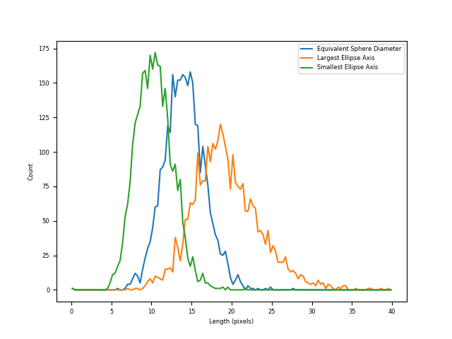
../_images/lab-F-particleSizeDist.png — Comparison of different measurements of particle diameters#

We can now choose one of these measurements (good luck choosing which one!) to generate a classic grain-size distribution image. For this we can use our internal plotter:

import spam.plotting

spam.plotting.plotParticleSizeDistribution(radii*15*4/1000.0, # Multiplying by pixel size in mm
                                           bins=256,
                                           units="mm",
                                           cumulative=True,
                                           cumulativePassing=True,
                                           mode="mass", # % passing by mass and not number of particles
                                           range=[0, 2],
                                           logScaleX=False,
                                           logScaleY=False)

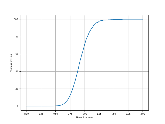
../_images/lab-G-particleSize.png — Particle size distribution#

Visualising label quantities#

Colouring particles/labels with some properties has become a common way to show things – see [Hall2010] for an early example. In this context we achieve this by converting a labelled image into an image where labels are replaced by some scalar. This could be any scalar field – since we have it handy, why don’t we colour grains by their longest half-axis? Let’s use the convertLabelToFloat function:

labelledMaxEllipse = spam.label.convertLabelToFloat(labelled, 2.0*ellipseAxes[:,0])
plt.imshow(labelledMaxEllipse[:, :, labelledMaxEllipse.shape[2]//2], cmap="plasma"); plt.colorbar(); plt.show()

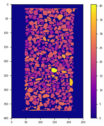
../_images/lab-H-relabelEllipseMax.png — Labelled image with labels replaced by max fitting ellipse lengths (in pixels)#

Discretising a labelled space#

There are two logical ways of separating the volume of a granular system into logical components:

Either through the pores: a Voronoi diagram

Or through the grains: a Delaunay Triangulation

One is the topological dual of the other. Here we use a convenient modification of the voronoi: the Set Voronoi, which is a modification proposed in [Schaller2013]. It has some nice properties, like never intersecting grains (always going through contacts), which is good news for irregular granular media. The edges of the Set Voronoi cells are not straight lines

However we will use SciPy’s Delaunay Triangulation (itself based on QHull libraries) so this is not quite the dual of the Set Voronoi. Let’s check out both:

setVoronoi = spam.label.setVoronoi(labelled)
# output:
#   Set Voronoi progress:           100.0%

# [1:] means keep only from label 1 onwards (*i.e.,* exclude the first 0,0,0)
centres = spam.label.centresOfMass(labelled)[1:]
# output:
#   Bounding box progress:          100.0%
#   Centres of mass progress:       100.0%

import scipy.spatial
delaunay = scipy.spatial.Delaunay(centres)
# This generates a delaunay object.
#   Let's pass this to a voxel labeller, it will return a
#   volume of the size of "labelled", with tetrahedra labelled
triangulation = spam.label.labelTetrahedraForScipyDelaunay(labelled.shape, delaunay)

# Let's see what we did:
plt.figure()

# We'll prepare 4 slices -- a full Set Voronoi:
setVoronoiSlice = setVoronoi[:, :, labelled.shape[2]//2].copy()
plt.subplot(2,2,1); plt.imshow(setVoronoiSlice, cmap=spam.label.randomCmap)
plt.title("Set Voronoi")

# A Set Voronoi with grains set to zero
setVoronoiSlice[labelled[:, :, labelled.shape[2]//2] != 0] = setVoronoiSlice.max()

plt.subplot(2,2,2); plt.imshow(setVoronoiSlice, cmap=spam.label.randomCmap)
plt.title("Set Voronoi minus grains")

# Same for Delaunay, full:
triangulationSlice = triangulation[:, :, labelled.shape[2]//2].copy()
plt.subplot(2,2,3); plt.imshow(triangulationSlice, cmap=spam.label.randomCmap)
plt.title("Delaunay Triangulation")

# ...and with holes
triangulationSlice[labelled[:, :, labelled.shape[2]//2] != 0 ] = triangulationSlice.max()
plt.subplot(2,2,4); plt.imshow(triangulationSlice, cmap=spam.label.randomCmap)
plt.title("Delaunay Triangulation minus grains")
plt.show()

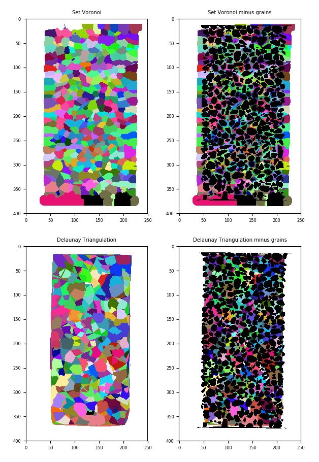
../_images/lab-I-setVoronoiAndTriangulation.png — (top left) Set Voronoi, (top right) Set Voronoi with grains subtracted, (bottom left) Delaunay triangulation, (bottom right) Delaunay triangulation with grains subtracted#

Not that easy to see in the end, but the Set Voronoi draws a nice contour around each grain, whereas the Delaunay triangulation has the centres of grains as the vertices of the tetrahedra.

It’s important to note that the labels of the grains are preserved in the Set Voronoi – essentially you can think of it as an expansion of each labelled grain.

Exercise for the reader: The Set Voronoi offers a convenient way to define the local void ratio for each grain – can you make a map of it?

References#

[Hall2010]

Hall, S. A., Bornert, M., Desrues, J., Pannier, Y., Lenoir, N., Viggiani, G., & Bésuelle, P. (2010). Discrete and continuum analysis of localised deformation in sand using X-ray μCT and volumetric digital image correlation. Géotechnique, 60(5), 315-322. https://doi.org/10.1680/geot.2010.60.5.315

[ITK2006]

Beare, R., & Lehmann, G. (2006). The watershed transform in ITK-discussion and new developments. The Insight Journal, 6. http://www.insight-journal.org/midas/bitstream/view/1157

[Ikeda2000]

Ikeda, S., Nakano, T. & Nakashima, Y. (2000). Three-dimensional study on the interconnection and shape of crystals in a graphic granite by X-ray CT and image analysis. Mineralogical Magazine, 64(5), pp. 945-959 https://doi.org/10.1180/002646100549760

[Schaller2013]

Schaller, F. M., Kapfer, S. C., Evans, M. E., Hoffmann, M. J., Aste, T., Saadatfar, M., … & Schröder-Turk, G. E. (2013). Set Voronoi diagrams of 3D assemblies of aspherical particles. Philosophical Magazine, 93(31-33), 3993-4017. https://doi.org/10.1080/14786435.2013.834389

Tutorial: Label Toolkit

Contents