
Tutorial: Strain calculation#
Objectives of this tutorial#
In materials science, it is of clear interest to obtain information about the deformation of the material rather than its displacement. A rigid-body displacement consists of a translation and rotation of the material without changing its shape or size, whereas a deformation implies change in shape and/or size of the material.
Strain is a description of this deformation, in terms of relative displacement of points inside the material, excluding any rigid-body motions. Therefore, a calculation of a strain field is necessary to describe the intrinsic material’s response to an external loading.
The aim of this tutorial is to:
describe the framework on which the strain field is calculated in spam, supported by basic notions of continuum mechanics
provide an example explaining how to use the script to calculate a strain field from a displacement field coming from a correlation
From a displacement field to a strain field#
In continuum mechanics, a common method for calculating strains, relies on the transformation gradient, which is the local characterisation of the motion. Local strains are computed based on a local variation in a displacement field (relative displacements of neighbouring points). It is thus natural to proceed with a strain calculation based on the displacement field resulting from the correlation process (following this part of the tutorial on Image Correlation).
Correction/filtering of the displacement field#
It should be noted that this operation is purely a mathematical derivation (i.e., calculation of gradient) of the displacement field and thus is very sensitive to errors/noise on the displacement field (see tutorial on errors, coming soon).
Furthermore, in the calculation of the displacement field, from spam-ldic, there is no imposed continuity between the displacements of the centre of each subvolume of the grid.
It can also happen that some of the points of the grid have not been correlated successfully (either they did not converge to the right solution or simply diverged; see this page).
For all these reasons, there is a `script`_ called spam-filterPhiField to correct the calculated displacement field by replacing each of the badly correlated points with a weighted influence of the closest good points and also smooth it, by applying a median filter.
The correction or filtering of the field is not obligatory, but sometimes highly recommended in order to end up with a strain field that makes sense.
Computing a Transformation Gradient Tensor, F#
In spam we have implemented two modes for computing the transformation gradient tensor F from a displacement field:
the Q8 shape function linking 8 neighbouring nodes as illustrated below and available in functionQ8
A slower but more flexible method developed by [GEE1996] which makes an average on a neighbourhood, and expresses F at the measurement points, available in functionGeers
In the case of the Q8 element, a linear coordinate mapping inside a Q8 element is performed and we are thus calculating a 3x3 transformation gradient tensor, F, at the center of the element defined as:
where I is the identity matrix and \(\nabla u\) is the gradient of the displacement vector.
Note that for the contribution of each node to be equally weighted, it is implied that the grid should be regular, but not necessarily equally spaced in all directions.
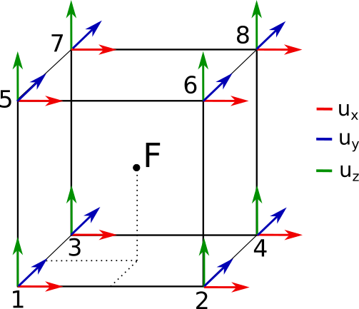
A Q8 element as part of the regular grid. The node convention differs from classical finite element due to the way nodes are retrieved from the larger grid. Note that the transformation gradient is computed in the centre of the element.#
The calculated transformation gradient tensor F has a clear physical meaning: local derivatives of the displacement, describing the deformation at neighbouring points. However, it contains components of the material rotations which do not represent any intrinsic material response to external loading. These rotations are seen as asymmetries in the transformation gradient, whereas, in a Cauchy continuum, symmetric components in F are equal. The decomposition of this tensor into strains and rotations is explained in details in Tutorial: Refreshments in continuum mechanics.
Strain invariants#
Having done a polar decomposition of F to end up with the stretch tensor U, it is useful now to decompose the strain tensor in an isotropic (i.e., spherical) and deviatoric part and extract scalars representative of the volume and shear distortion of the material at that point, respectively. For more details, please have a look at these very helpful notes by Denis Caillerie.
A multiplicative decomposition of the symmetric stretch tensor U is used:
where J is the determinant of the transformation gradient tensor and D the dimensions of the problem.
As a first invariant of the strain tensor, the volumetric strain is defined as:
As a second invariant of the strain tensor, the deviatoric strain can be defined as the Frobenius norm of the deviatoric part:
Small strain approximation#
What has been presented above, is a general framework known as large (finite) strain theory. In cases where the relative displacements of the material points are assumed to be much smaller (infinitesimally smaller) than any relevant dimension of the material, the small (infinitesimal) strain theory is adopted as a mathematical approach for the description of the deformation of the material. With this assumption, the equations of continuum mechanics are considerably simplified.
In the small strains framework, we can assume that the rotations are negligibly small and define the strain tensor as:
Actually, by adding the F tensor and its transpose, we are getting rid of the asymmetry caused by the rotations; however the rotation components will be still misinterpreted as strain, introducing an error in the strain tensor.
In small transformations, a transformation is composed by adding the displacements. Thus, an additive decomposition of the small strain tensor ε can be used:
where D are the dimensions of the problem.
As a first invariant of the small strain tensor, the volumetric strain can be defined as:
Similarly with the large strains, as a second invariant of the small strain tensor, the deviatoric strain can be defined as the euclidian norm of the deviatoric part:
Keeping in mind that it is always correct to use the large strains definition, it can easily be proven that small strains is an approximation of large strains:
where:
are, respectively, the anti-symmetric and symmetric parts of \(\nabla u\).
We can note that the inherent difference between the two definitions resides in the way successive transformations are followed: by an additive process in small strains and a multiplicative process in large strains.
Example: Let’s calculate a strain field#
Now it’s time to run the suitable script to calculate our strain fields.
Following the framework described above, the script_ computes a strain field based on a given displacement field calculated at a regular grid.
It takes as input a TSV file, which is a result from a spam-ldic correlation.
The options include:
the choice of method to calculate the transformation gradient (Q8/Geers),
the choice of framework to calculate strains (small/large),
the desired strain invariants,
an option for excluding nodes based on the correlation return status (see note below)
and of course the desired output files
By default, the framework is the large strains approximation. By default, only nodes that have a Return Status = 2 are considered for the calculation.
Important tip:
If you have applied a median filter at your field, the Return Status of the nodes has automatically changed from RS = 2 to RS = 1.
This means that you need to run the strain script adding this option to change the return status threshold: -rst 1
Again, the full options are available with the -- help command.
We are going to calculate the strains coming from the measured displacement field of this example.
Let’s look at the example running the strain script with different options:
First we will compute the strain field under the hypothesis of large strains using Q8 element.
bash> source venv/bin/activate
(venv)bash> spam-regularStrain                   # The script
                VEC4-01-b1-VEC4-02-b1-ldic.tsv \ # The tsv (result of ``spam-ldic``) to load
                -tif -vtk \                      # Ask for TIFF file and VTK output
                -comp vol dev U \                # Ask for strain invariants and stretch tensor
                -cub                             # Ask to calculate F with a Q8 element. If not given, the default option (Geers) is applied
This time, the strain script will compute the strain field using Q8 element under the hypothesis of small strains, meaning that for every point in the field the strain tensor ε is computed.
bash> source venv/bin/activate
(venv)bash> spam-regularStrain                   # The script
                VEC4-01-b1-VEC4-02-b1-ldic.tsv \ # The tsv (result of ``spam-ldic``) to load
                -tif -vtk \                      # Ask for TIFF file and VTK output
                -comp volss devss e \            # Ask for small strain invariants and small strain tensor
                -cub                             # Ask to calculate F with a Q8 element. If not given, the default option (Geers) is applied
The 6 components of these symmetric tensors are saved as independent tiff files, together with the volumetric strain (first invariant of the strain tensor) and the deviatoric strain fields (second invariant) of the strain tensor. Also, the strain fields (with all its components) have been saved as a vtk format (for a 3D visualisation in ParaView).
The volumetric strain can be positive or negative, with 0 meaning no volume change. We use mechanical engineering convention (and not soil mechanics convention) meaning that compressive strains are negative.
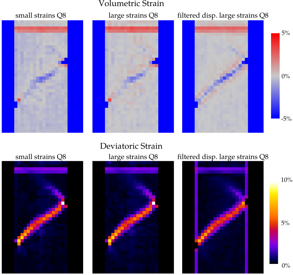
Central vertical slices through the first and second invariants of the locally-measured strain fields under the hypothesis of small and large strains. Third column results from a median filtered displacement field with a radius of 1 pixel.#
It seems that there is a slight difference between the choice of framework and that the filtering of the displacement field results, as expected, in a smoother strain field. The calculated strain fields reveal clearly a shear band crossing the sample between the manually-created notches, with a wing-crack appearing to start also from one notch.
Visualising the deviatoric strain field in ParaView (hiding strain values below 0.8% which appears to be the background noise level for this particular measurement) yields an interesting field:
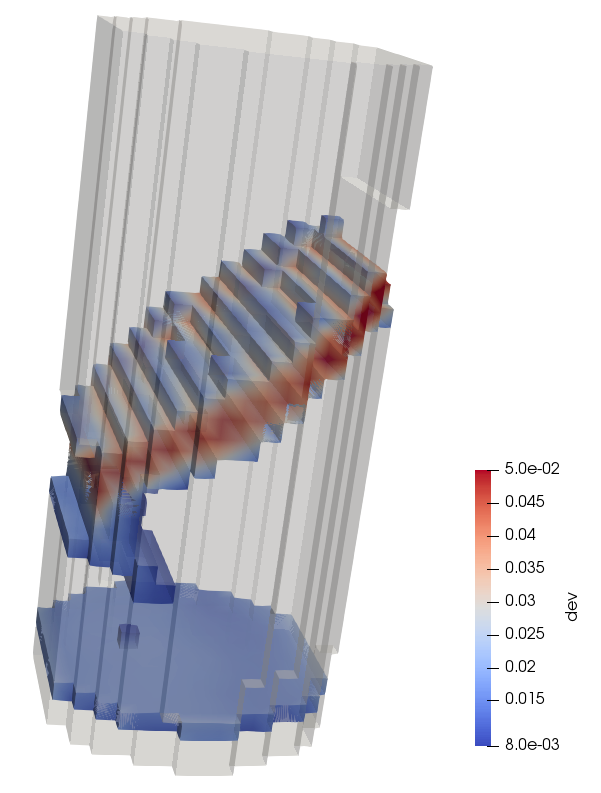
3D visualisation of the deviatoric strain field, hiding values below 0.8% strain#
Clarification: Deformation Function Φ vs Transformation Gradient Tensor F#
It should be mentioned that a confusion may arise from the definition of this transformation gradient F. Following the Tutorial: Image correlation – Theory, a transformation matrix was also introduced, however of dimensions 4x4 that we call Φ. From a continuum mechanics point of view, the two tensors are equivalent. Φ is an extension of F taking into account also the translation vector, which together with the rotations describe the rigid-body motion of the material.
However, the method of calculating these two tensors is different. Φ describes the transformation of the correlation window (CW) applied directly on the initial signal to match the signal of the second image. After having obtained Φ, a polar decomposition is used again, to separate the (3x3) top-corner submatrix to the resulting deformation (as explained in details here).
However, this resulting deformation can accumulate large errors due to noise or degradation of the local greyvalues between the two images. Nonetheless, the correlation process could still capture meaningful displacements. It is thus deemed preferable to calculate strains from the relative point displacements rather than from the deformation of the CW.
Having said that, it is quite interesting to plot the two deformation tensor fields and examine their differences.
We’re going to plot the first and second invariants of strain obtained by decomposing F which has come from three different sources:
decomposing the stretch tensor coming directly from the Φ of the subvolume as a result of the correlation
by deriving the displacement field resulting from the same correlation with Q8 elements
from the Geers formulation
Here’s the script to do it:
import numpy
import spam.helpers
import spam.DIC
import spam.deformation
import spam.mesh
import matplotlib.pyplot as plt

plt.rcParams.update({'font.size': 20,'axes.labelsize':20,'axes.labelpad':20, 'xtick.major.pad':10,'ytick.major.pad':10,'legend.fontsize':12, 'text.usetex': True,       'font.weight':'bold','axes.labelweight':'bold'})

# read the result of the correlation
DVC = spam.helpers.readCorrelationTSV("VEC4-01-b1-VEC4-02-b1-ldic.tsv")

PhiFieldDVC = DVC['PhiField'].reshape(DVC["fieldDims"][0], DVC["fieldDims"][1], DVC["fieldDims"][2], 4, 4)
spaceX = DVC["fieldCoords"][1,2] -                                       DVC["fieldCoords"][0,2]
spaceY = DVC["fieldCoords"][DVC["fieldDims"][2],1] -                     DVC["fieldCoords"][0,1]
spaceZ = DVC["fieldCoords"][DVC["fieldDims"][2]*DVC["fieldDims"][1],0] - DVC["fieldCoords"][0,0]

strainComponents = ['vol', 'dev']

### First compute vol and dev from the locally-measured Phi
decomposedFfieldLocal = spam.deformation.decomposeFfield(PhiFieldDVC[:, :, :, 0:3, 0:3], strainComponents)

### Second, compute F from Q8 elements, and then the vol and dev components
FfieldQ8 = spam.deformation.FfieldRegularQ8(PhiFieldDVC[:, :, :, 0:3, -1], [spaceZ, spaceY, spaceX])
decomposedFfieldQ8 = spam.deformation.decomposeFfield(FfieldQ8, strainComponents)

### Third, compute F from Geers formulation, and then the vol and dev components
FfieldGeers = spam.deformation.FfieldRegularGeers(PhiFieldDVC[:, :, :, 0:3, -1], [spaceZ, spaceY, spaceX])
decomposedFfieldGeers = spam.deformation.decomposeFfield(FfieldGeers, strainComponents)

volVmin = -0.025
volVmax =  0.025
devVmin = 0.0
devVmax = 0.05

plt.subplot(2, 3, 1)
plt.title("vol -- Local")
plt.imshow(decomposedFfieldLocal['vol'][:,DVC["fieldDims"][1]//2], vmin=volVmin, vmax=volVmax, cmap='coolwarm')
plt.colorbar()

plt.subplot(2, 3, 2)
plt.title("vol -- Q8")
plt.imshow(decomposedFfieldQ8['vol'][:,DVC["fieldDims"][1]//2], vmin=volVmin, vmax=volVmax, cmap='coolwarm')
plt.colorbar()

plt.subplot(2, 3, 3)
plt.title("vol -- Geers")
plt.imshow(decomposedFfieldGeers['vol'][:,DVC["fieldDims"][1]//2], vmin=volVmin, vmax=volVmax, cmap='coolwarm')
plt.colorbar()

plt.subplot(2, 3, 4)
plt.title("dev -- Local")
plt.imshow(decomposedFfieldLocal['dev'][:,DVC["fieldDims"][1]//2], vmin=devVmin, vmax=devVmax, cmap='plasma')
plt.colorbar()

plt.subplot(2, 3, 5)
plt.title("dev -- Q8")
plt.imshow(decomposedFfieldQ8['dev'][:,DVC["fieldDims"][1]//2], vmin=devVmin, vmax=devVmax, cmap='plasma')
plt.colorbar()

plt.subplot(2, 3, 6)
plt.title("dev -- Geers")
plt.imshow(decomposedFfieldGeers['dev'][:,DVC["fieldDims"][1]//2], vmin=devVmin, vmax=devVmax, cmap='plasma')
plt.colorbar()

plt.show()
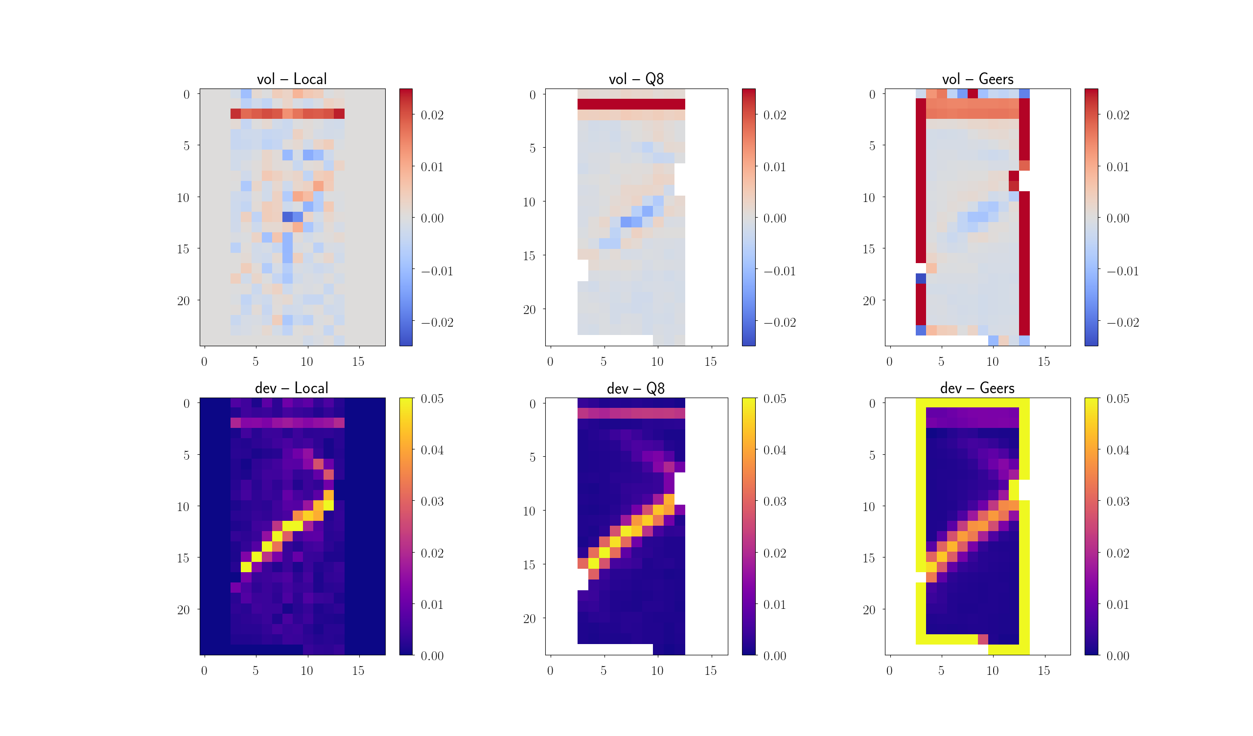
Central vertical slices through the first and second invariants of the decomposed stretch tensor field. On the left coming directly from the measured Φ of each subvolume as a result of the correlation – this is very noisy but the most local. In the middle F is computed by linking 2×2×2 neighbourhood displacements with a Q8 element. On the right coming the [GEE1996] formulation is used to obtain F#
As it was expected, the local stretch tensor field (coming directly from the transformation of the subvolume in the correlation) is finer, but noisier. It seems to be a clear noise/spatial resolution trade-off between the different ways of obtaining the stretch tensor fields.
References#
Geers, M. G. D., De Borst, R., & Brekelmans, W. A. M. (1996). Computing strain fields from discrete displacement fields in 2D-solids. International Journal of Solids and Structures, 33(29), 4293-4307. https://doi.org/10.1016/0020-7683(95)00240-5