The objective of this tutorial is to measure particle kinematics (i.e., particle tracking) with the scripts available in spam.
Unlike the local (regular cuboids) or global (continuous mesh) DVC techniques, the objective here is to measure a Φ for each particle.
This is done by solving the DVC problem for the greyscales corresponding to the particle, which are conveniently defined by masking the greyscale image with the labelled image (see Tutorial: Label Toolkit) where each particle has a unique number.
Using the terminology in Tutorial: Image correlation – Theory, here ROI will be the greyscale values associated with each particle’s labelled voxels.
This “Discrete DVC” approach was first discussed in [Hall2010], and re-implemented in [Ando2013] to measure particle rotations after an initial tracking.
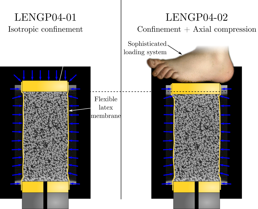
The example we will use is from Gustavo Pinzón’s PhD work: repeated x-ray tomography scans as a cylinder full of lentils initially oriented at 45° is deformed in triaxial compression.
Please use this link and download all the data (and folder structure) for this tutorial.
The experiment is called LENGP04 and has a (large) number of scans labelled sequentially during loading.
The first scan is under isotropic compression, the next ones are with increasing axial shortening.
Here are vertical sections through the first two scans:
Experience shows that Discrete DVC is enormously facilitated by having a labelled volume which is faithful to the data.
In this example we will used a pre-cooked labelled volume coming from the ITK watershed offered in spam with some manual post-processing.
As should be clear in the DVC theory tutorial, the image gradients are important, and so in this case it is important the the labelled image catches the greylevels corresponding to the edges of the particles.
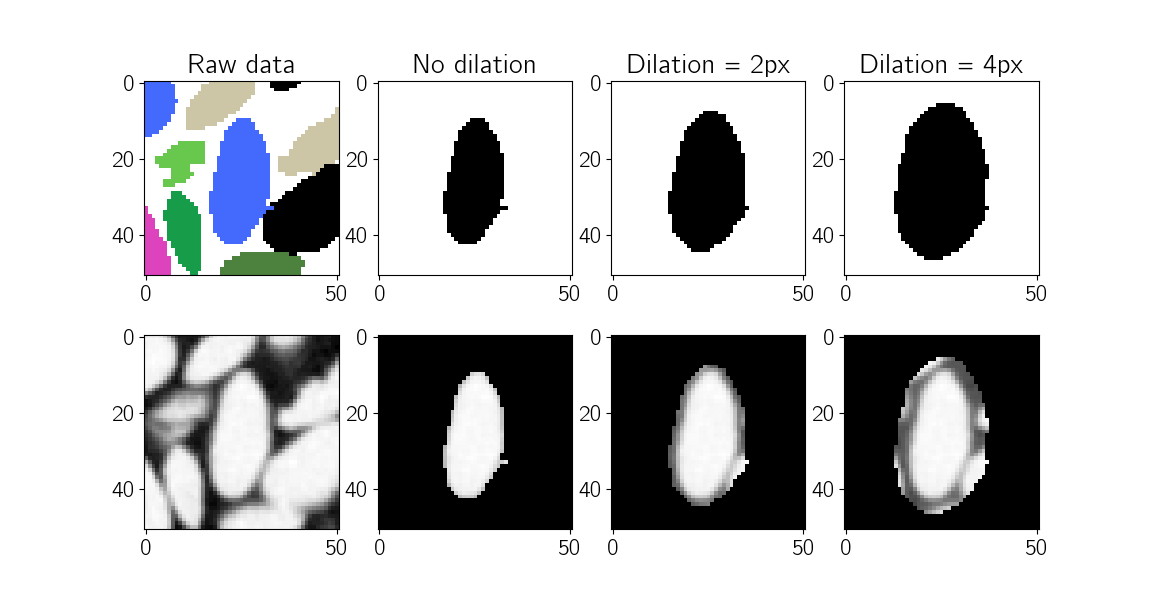
For this reason the label for each particle can be gently dilated to make sure the greylevel falloff at the edges of the particles are captured.
Here’s an example with a single lentil:
“No dilation” is cutting probably too close to the edge. If your particles have internal texture, this would be fine, but as you can see in this case the lentil is pretty flat.
One or two pixel dilation is probably fine in this case, and as you can see the 4px dilation includes a lot of parts of other particles and thus will thus pollute the quality of the kinematics measurement – in some instances we have observed convergence of the DiscreteDVC only on the neighbours, which is not what is desired here. Don’t dilate too much.
Since it’s often quite hard work to get a great labelled image, in this tutorial we will choose to only use the label image of the initial scan and perform total correlations, meaning that we will correlate from t=0→1 then t=0→2 and t=0→3 (but of course using the information t=0→1 to help with t=0→2, etc.).
Just like spam-ldic from spam 0.6 onwards, the spam-ddic represents the iterative Newton algorithm to make a fine Φ measurement, and thus needs to start close to the correct solution .
spam > 0.6 offers 2 main ways to get this:
An overall registration of the entire greyscale volume.
This works well for small increments that are relatively homogeneous).
You can then give the TSV containing the measured overall deformation function Φ to spam-ddic.
Or a brute-force displacement-only search called a pixel search.
This will extract each grain and search around for it (displacement only) in the deformed image, looking for the displacement that gives the best Normalised Correlation Coefficent value (i.e., the closest to 1.0).
You can then give the TSV containing the measured displacement to spam-ddic.
In this example we will use a pixel search – it needs to know how far to search.
Since the search is brute force the further you search the longer it takes.
We judge by eye that the top cap is moving down 7 pixels in the +z direction, and that the bottom cap is not moving at all. We therefore we should set the search range to have ±1 pixel safety margin in the z-direction and ±4 pixels in x and y.
However we are also going to purposely make a mistake and only look 3 pixels in the Z direction
This will create “00-01-good/bad-pixelSearch.tsv/vtk” in the PS folder.
Keep an eye on the Correlation Coefficient values that are outputted during the pixel search, they should be close to 1.00.
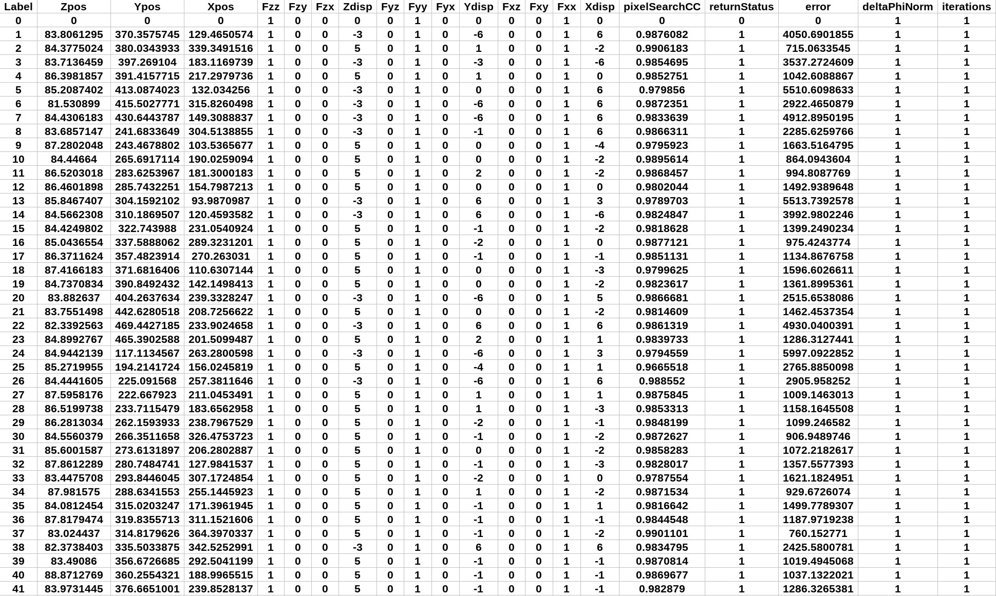
After running this (a few minutes), you will get a TSV file.
What needs to be checked is that this is as high as possible – meaning that we have searched far enough to match the particles.
IMPORTANT POINT: for reasons of alignment we keep label 0 – the background in the output TSV file.
We’ll exclude it when we analyse things.
There are a few ways to check out TSV output:
Load the TSV as a spreadsheet (drag and drop it into Libreoffice Calc, or Excel if you dare).
look for low CC values, this is not really recommended.
Load the TSV in ipython have a look around (the [1:] is to avoid the 0.0 CC for label ):
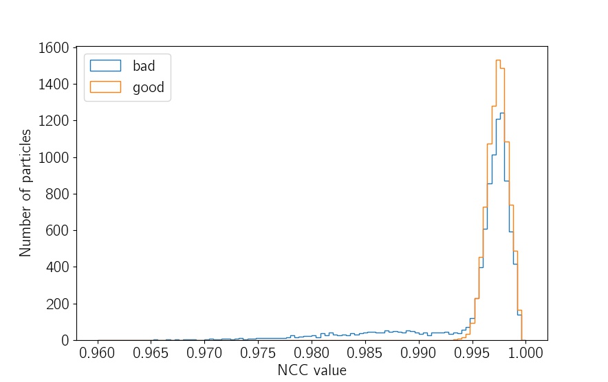
importspam.helpersimportnumpyPSbad=spam.helpers.readCorrelationTSV("PS/00-01-bad-pixelSearch.tsv",readPixelSearchCC=1)PSgood=spam.helpers.readCorrelationTSV("PS/00-01-good-pixelSearch.tsv",readPixelSearchCC=1)print("Minimum and Average CC value for bad correlation")print(numpy.min(PSbad['pixelSearchCC'][1:]))print(numpy.mean(PSbad['pixelSearchCC'][1:]))print("\nMinimum and Average CC value for good correlation")print(numpy.min(PSgood['pixelSearchCC'][1:]))print(numpy.mean(PSgood['pixelSearchCC'][1:]))# -- Output --# Minimum and Average CC value for bad correlation# 0.9498977# 0.9952788277559265## Minimum and Average CC value for good correlation# 0.9916541# 0.9973577603805677
Other than that the distributions of CC values could also easily be compared:
importmatplotlib.pyplotaspltplt.hist(PSbad['pixelSearchCC'][1:],bins=100,range=[0.96,1.0],label='bad',histtype='step')plt.hist(PSgood['pixelSearchCC'][1:],bins=100,range=[0.96,1.0],label='good',histtype='step')plt.legend(loc='upper left')plt.xlabel("NCC value")plt.ylabel("Number of particles")plt.show()
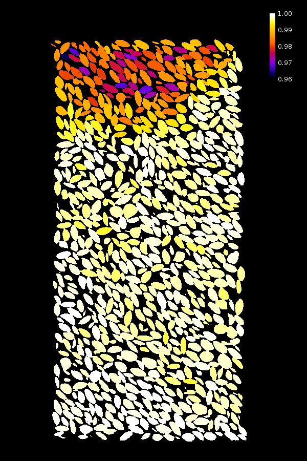
…or for more advanced use, convert your labelled image to show CC values:
This colours all particles by their CC value, giving a map like this:
This representation is helpful to understand the spatial organisation of any property (in this case the CC values of Pixel Search). As you can see, the lower values (below 0.99) correspond to the particles near the top cap, and are a result of our deliberated selection of the wrong PS range.
Visualise with paraview
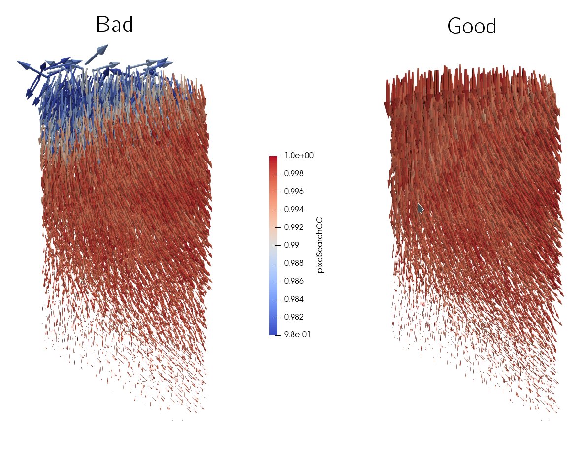
Drag and drop VTK file into Paraview and do “Apply” → Generate Glyphs → “Scale mode” = “vector” AND “Glyph Mode” = “All Points” → Colour vectors by pixelSearchCC.
This gives a vector field where arrows show the displacement and are coloured by the CC value:
Eventhough we might think that values below 0.99 are good enough, we can observe that the measured displacement can not be trusted.
This will create “00-01-ddic.tsv/vtk” in the DDIC folder.
Here there will be two main questions: did each particle’s correlation converge? And if so, did it converge to the correct solution?
In order to see the convergence, we need to look at the “return status” (RS) of each particle (see the scripts documentation for their exact meaning Discrete local DIC script (spam-ddic)).
Convergence is RS=2, Hitting max iterations is RS=1, and anything negative is bad.
As before you can load the resulting TSV or VTK files in any way you like, let’s do it in ipython:
DDIC=spam.helpers.readCorrelationTSV("DDIC/00-01-ddic.tsv")unique=numpy.unique(DDIC["returnStatus"][1:],return_counts=1)forrs,numberinzip(unique[0],unique[1]):print(f"{number} particles have Return Status={rs}")# -- Output --# 2 particles have Return Status=-1.0# 1 particles have Return Status=1.0# 9404 particles have Return Status=2.0
Three particles have not coverged properly. This is not a disaster, but it is recoverable, so let’s try to make them work.
The Φ current saved in the TSV is now corrupted, and so should be reset.
Let’s do this by interpolating the Φ from converged neighbours
This will create “00-01-ddic-filtered.tsv” in the DDIC folder.
-srs means “select points to filter based on return status” and -cint means “correct based on a local interpolation”.
This creates a new file called DDIC/00-01-ddic-filtered.tsv.
Let’s run a new DDIC with two new options:
-skp: runs DDIC only on the four non-converged particles, (i.e., skipping RS==2 )
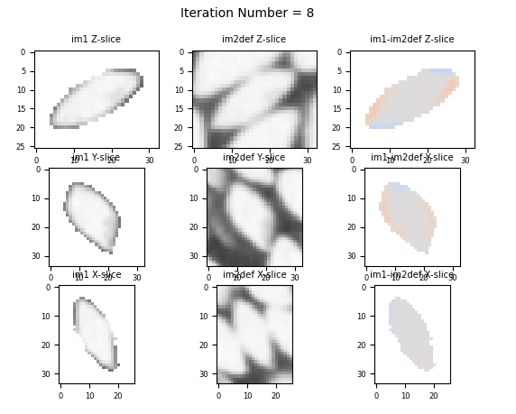
-d: activates debug mode and allows us to follow the correlation progress graphically (this needs to run in single-process mode, and combined with the graphical output is very slow, not recommended for more than a few particles)
This will overwrite “00-01-ddic.tsv/vtk” in the DDIC folder.
Here’s what the debug window looks like:
Weird they don’t converge nicely, despite being practically in the right place.
Often the correlation needs more information or more flexibility.
Here are some hints to help it converge:
-nr: makes the correlation more flexible, and allows the Φ to be non-rigid
increase -ld: can add a bit of extra edge information, don’t make it too big!
-ug: Slow down computation by making the correlation process Newton instead of Quasi-Newton
Let’s just activate -nr. Please redo the filtering step above (spam-filterPhiField) to reset Φ, then run
Again, this will overwrite “00-01-ddic.tsv/vtk” in the DDIC folder.
All the particles have now converged – meaning that the DDIC Newton algorithm has converged.
This is usually a good sign, but it is quite possible that poor solutions have been found – this is a reason why it’s not a good idea just to increase the number of iterations for DDIC until it converges: difficult convergence is a sign of a bad initial guess.
There are a number of ways that the quality of this final series of Φ functions can be checked – for example collisions could be detected.
Here we propose to apply the measured Φ function measured for each particle to the labelled image.
It’s important to stress that the labelled image is only defined to the nearest pixel.
We will use the spam-moveLabels script, which will generate the deformed labelled image.
It’s important to say that if there are collisions, labels will be overwritten in an uncontrolled way
This generates LENGP04_01-lab-moved.tif, which can be compared to the deformed greylevel image (LENGP_01) that was acquired.
Here we show a central vertical slice through the state LENGP04_00 (with acquired greylevels and labels) as well as LENGP04_01 (with acquired greylevels and moved labels). Note that label values/colours are preserved between steps:
The correspondence – at least on this slice – looks good.
We generally apply a threshold to the deformed greylevel image and compute the pixel coverage of the labelled image.
Let’s say that scrolling through the slices we see no badly placed particles, and let’s validate the measured Φ functions for each particle in DDIC/00-01-ddic.tsv.
Just like in the previous increment, we will use a pixel search to get a rough displacement guess.
However we will load the the 0→1 Φ functions, meaning that the search for each particle will be around its previous location.
spam-pixelSearch will also apply the previously-measured rotation for the search, which is very important in granular materials.
As before, we run the pixel search, updating the deformed image, and loading the DDIC TSV file
As you can see, the process can be easily automatic.
In order to save some time typing the same commands every time, we can set some variables on the terminal and run all the codes for a given step.
First, we define the variable DEF (the number of the defomed scan that we are trying to track), and create DEFs (a zero-padded string) along with the previous step DEFsP (zero-padded string of the previous step).
Given that the naming system we used in our images is LENGP04_00,LENG04_01,…LENGP04_15, etc, we need to match it as well when running the codes. The variables DEFs and DEFsP are formated to match the naming system.
See that the only input is the variable DEF, all the others are generated automatically.
You can just re-run this previous line to update DEF from step to step.
As before we can now run the pixel search,
This process is repeated until all the particles converge and we can move on to the next step.
Spoiler alert: Step 0→5 has one particle which doesn’t converge#
Once we reach the step 0→5, we observe that after all the previous steps there is still a particle that doesn’t converge. We will use the spam-ereg-discrete script, which allow us to manually set the guess for diverged particles.
This is most likely due to this particle rotating more than its neighbours, so that the interpolation of Φ in spam-filterPhiField doesn’t give a good enough guess.
Perhaps resetting the rotation part of Φ to the previously-measured rotation would be a better guess, but a little harder in this context.
As above let’s set first the variables on the terminal
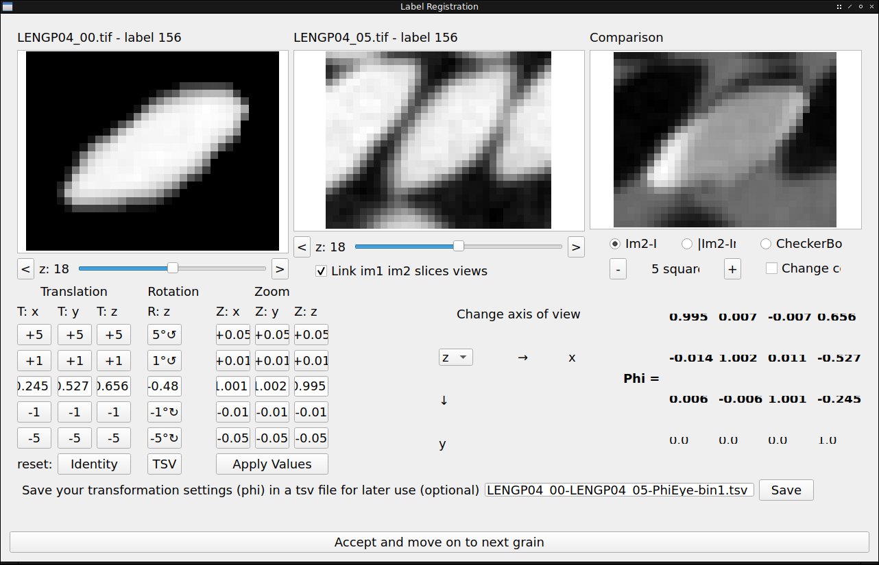
This pops up a window like this one, for all non-converged labels in the passed TSV file.
Remember to filter the TSV (or reset it to the previous converged state) before running the script, otherwise the starting position will be too far way from the correct solution and the script will be useless.
Here you can see the particle in the reference configuration (with the label applied as a mask – this can be disactivated with -nomask), the deformed image and a comparison (here you see the subtraction between the two images).
Since this particle can’t converge for some reason, you need to use the buttons, especially the translations and rotation, to align the particles.
A few hints:
Use all three “axes of view” to align your particle in 3D, you can loop over them using the drop-down menu under “Change axis of view”.
The direction of translation that will be applied to the reference state under the “axis of view”.
Rotations are applied around the current axis of view
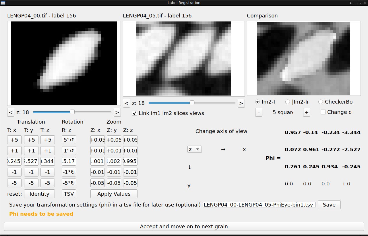
Here’s a reasonable effort – remember it doesn’t need to be perfect, just close enough for the DDIC to converge:
When you’re happy, press “Accept and move on to next grain” – here there is only one non-converged particle, so pressing the button will close the window and save the file “00-05-ereg-discrete.tsv”.
We can now use this as the initial guess for the (single) missing particle, and run spam-ddic again with -skp
As observed the tracking of particles is a process that follows some simple steps and that can be done iteratively.
The main points to follow are:
DDIC will perform better if we feed it with an initial guess. spam-pixelSearch can be used for this matter, coupled with the TSV file from the previous step.
Run spam-ddic and filter the result for the diverge particles. Multiple options as -nr, -ld, and -ug can be used to help the convergence of particles - remember to always use -skp when running again to compute only the diverged particles. Increasing the number of iterations is not always a good idea.
The script spam-ereg-discrete can be used to manually build the guess for stubborn particles that evade all our previous tools - this should be used only as a last resort.
In this example, tracking until step 09, the following vector plot can be obtained by dragging and dropping the series of VTK files in DDIC/, and rendering the displacements as glyphs.
This shows just the displacement although here the full (and total) Φ function has been measured for each particle.
What can we do with this information? A natural question is computing total strains.
Incremental strains would also be possible, but need to be computed between the correlated steps.
Here we will quickly illustrate two different methods for computing total strains, which will be expressed in the non-moving reference configuration.
We will chose to show the deviatoric (“maximum shear”) strain.
The most classical way to compute strains in a granular assembly is with a Delaunay triangulation of grain centres, using Bagi’s method [BAG1996].
The spam-discreteStrain script can also load the labelled image in order to compute particle volumes to have a Radical (weighted) Delaunay triangulation also known as a Laguerre tesselation – in this case particle sizes are very uniform, but it doesn’t cost much.
We have implemented one of the large strain formulations in [ZAN2015].
Let’s run spam-discreteStrain an all the DDIC TSV output files, and save the results in “strainTet” folder
(spam)$ forfileinDDIC/*ddic.tsv; do spam-discreteStrain -od strainTet -a 300 -rl LENGP04_00-lab.tif $file -tri; done
Loading all the resulting VTKs into paraview, then cutting them in half with with crinkle clip, shows an interesting pattern of total deviatoric strain:
For looking at deformation maps, we have found that it can be easier to project grain displacements onto a regular grid and use the spam-regularStrain computation.
We will therefore start by passing the discrete displacements onto a regular grid.
For this we need to make the script aware of the image size, and the node-spacing to define the grid.
There are a number of key options here for the interpolation of the discrete Φ onto the grid (whether to use all particles within a radius, or a fixed number of neighbours?), here we will accept the default
Zhang, B., Reguiero, R. A. (2015) On large deformation granular strain measures for generating stress–strain relations based upon three-dimensional discrete element simulations. International Journal of Solids and Structures, 66, 151-170
https://doi.org/10.1016/j.ijsolstr.2015.04.012