
Tutorial: Projection of morphologies onto a FE mesh#
Objectives of this tutorial#
In this tutorial we are going to project a morphology based on a tomographic 3D image of a concrete sample onto an unstructured mesh that could later be used for a Finite Element analysis that explicitly takes into account the heterogeneous aspect of the material.
The method used here is a non-adapted meshing technique (in opposition to conform meshes), which means that the resulting mesh will have some elements that belong to several phases. Such feature will eventually lead to discontinuity within the material properties to consider. See [Roubin2015] for an example of FE implementation using the Embedded Finite Element Method.
The several steps are:
- Starting with raw x-ray image and identifying the different phases of it
Applying filters to improve the quality and identify the phases
Using a mask to ignore the outside of the specimen
- Project the morphology onto the unstructured mesh
Construct the raw initial unstructured mesh
Compute the needed distance fields of each phase
Project the field onto the mesh
The obtained mesh contains the following features:
Repartition of phases for each elements
Orientation of the interface between phases for elements that belong in two phases and the corresponding subvolumes.
Step 1: Getting the repartition of phases#
The data used in this tutorial came from [Stamati2018b]. Please download c01_F10_b4.tif from spam tutorial archive on zenodo.
$ wget https://zenodo.org/record/3888347/files/c01_F10_b4.tif
Step 1.0: Load all python modules#
import tifffile
import matplotlib.pyplot as plt
import numpy
import spam.mesh
import spam.filters
Step 1.1: Load the data#
The image can be loaded using the classical tifffile library as follows:
im = tifffile.imread("c01_F10_b4.tif")
# Output:
# Image dimensions:
#         in z: 400
#         in y: 250
#         in x: 250
# Image encoded type: uint16 (which means unsigned integer encoded on 16 bits (4 bytes))
# Image greyscale:
#         Minimum value: 0
#         Maximim value: 65520
The horizontal slice in the middle looks like:
plt.imshow(im[im.shape[0] // 2], cmap="Greys")
plt.colorbar()
plt.title("Horizontal slice of the raw data")
plt.show()
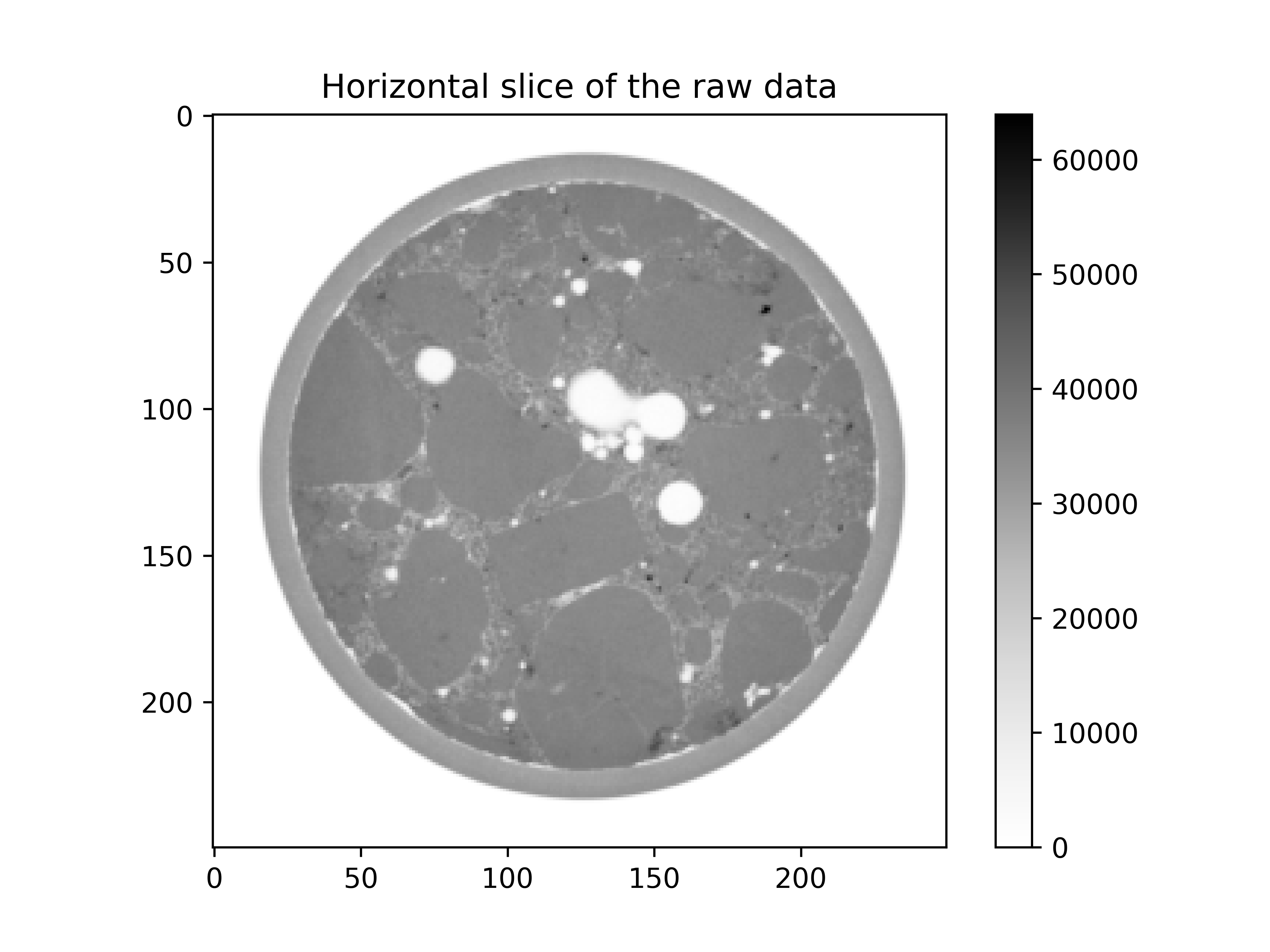
By eye we can easily identify the three phases of interest:
The aggregates: highest grey values and homogeneous structure
The mortar matrix: high grey values and rather heterogeneous structure
The voids: grey values close to zero.
The outside (which is also close to zero) and the membrane will be ignored with a mask.
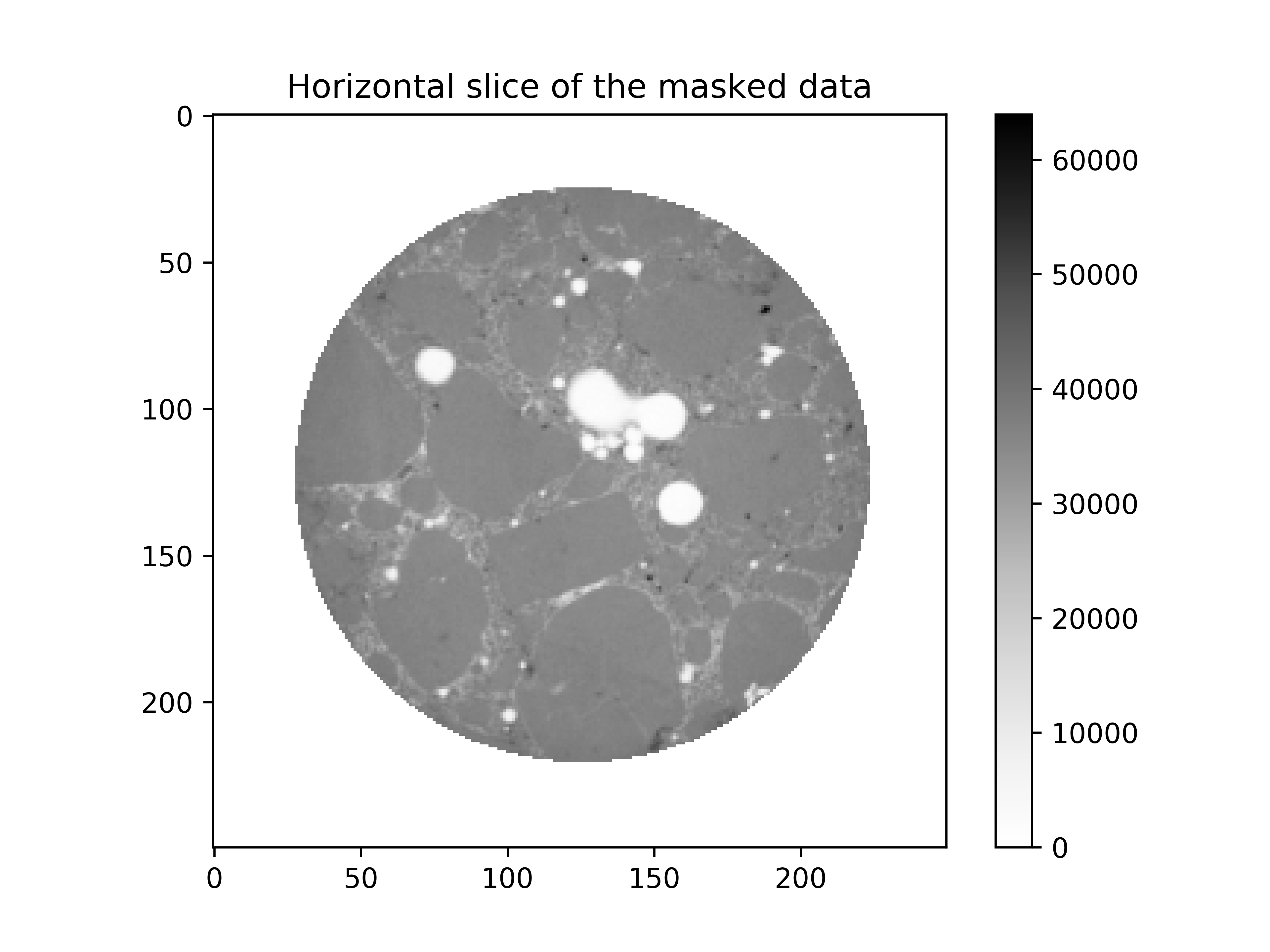
Step 1.2: Creation of a mask#
We start to create cylindrical mask in order to ignore the membrane. Then, with this mask we set the outside and the membrane to 0:
# create mask
mask = spam.mesh.createCylindricalMask(im.shape, 98, centre=[123, 126])
# set outside + membrane to 0
im = mask * im
# identification of the pores
pores = (im < 20000) * mask
# application of the filter
plt.imshow(im[im.shape[0] // 2], cmap="Greys")
plt.colorbar()
plt.title("Horizontal slice of the masked data")
plt.show()
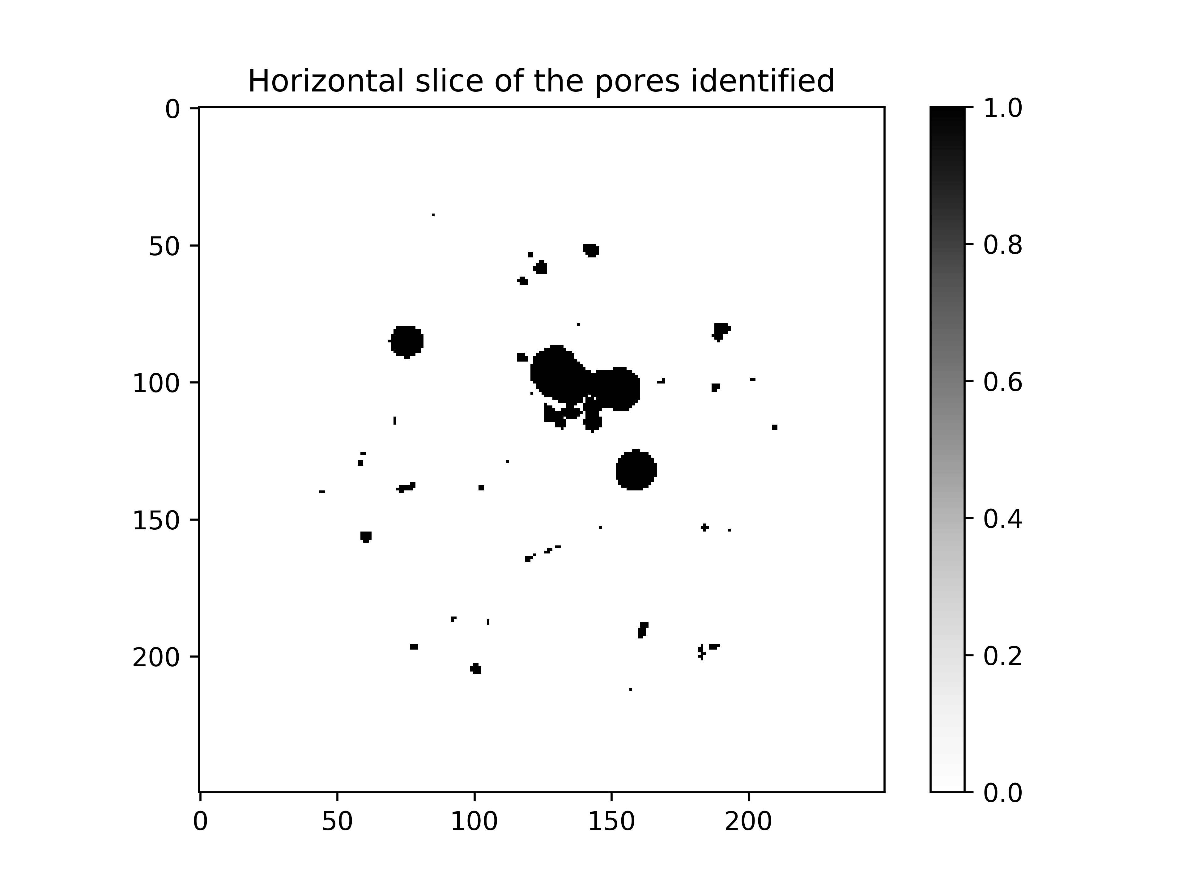
Step 1.3: Pores identification#
The pores can now be identified by setting everything that is below the grey value 20000 to 1 and the rest to 0. The mask is still used since the outside is now set to 0:
# identification of the pores
pores = (im < 20000) * mask
plt.imshow(pores[pores.shape[0] // 2], cmap="Greys")
plt.title("Horizontal slice of the identified pores")
plt.show()
Step 1.3: Aggregates identification#
The identification of the aggregates is a bit trickier since the grey value is close to the one of the mortar matrix. For this reason the threshold is made on the image after the application of a variance filter (or standard deviation):
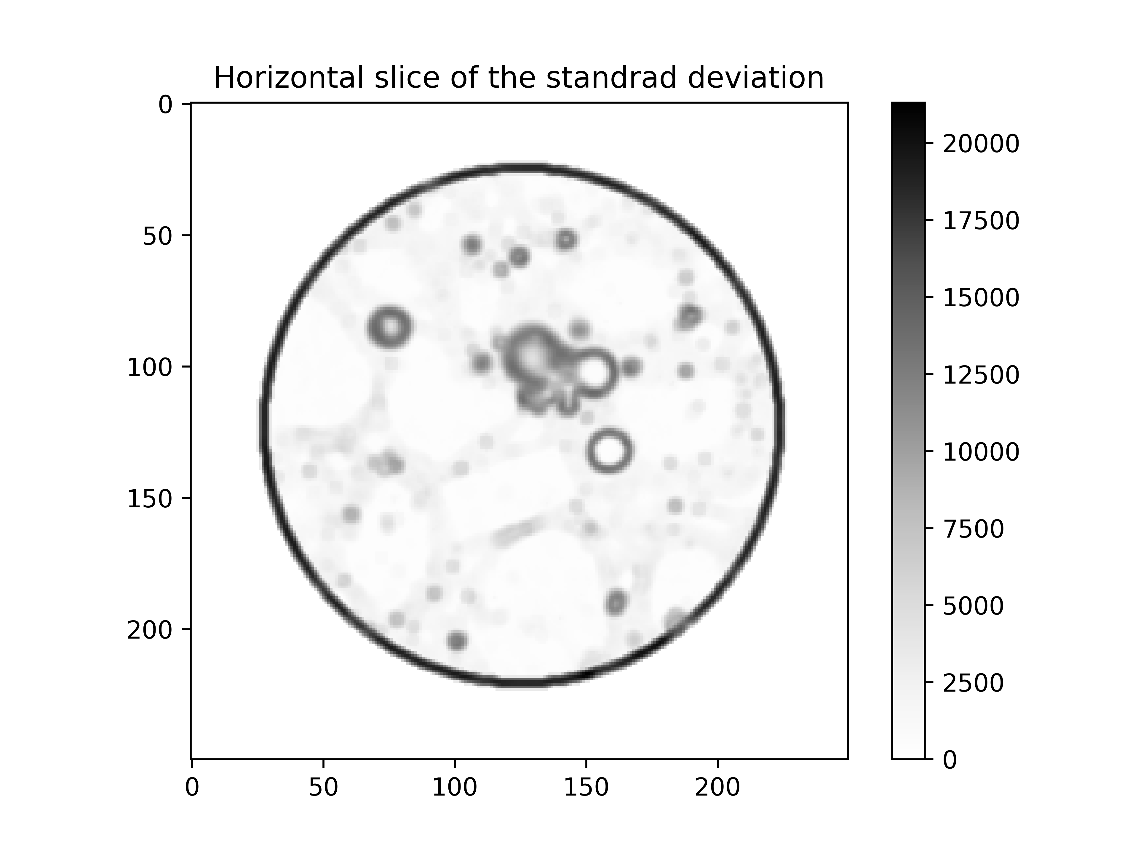
The low variance regions (aggregates and pores) are kept by thresholding the filtered image and the already identified pores are discarded:
# keep the values lower than 1090
aggregates = (standardDev < 1090) * mask
# then set the previously identified pores to 0
aggregates[pores == 1] = 0
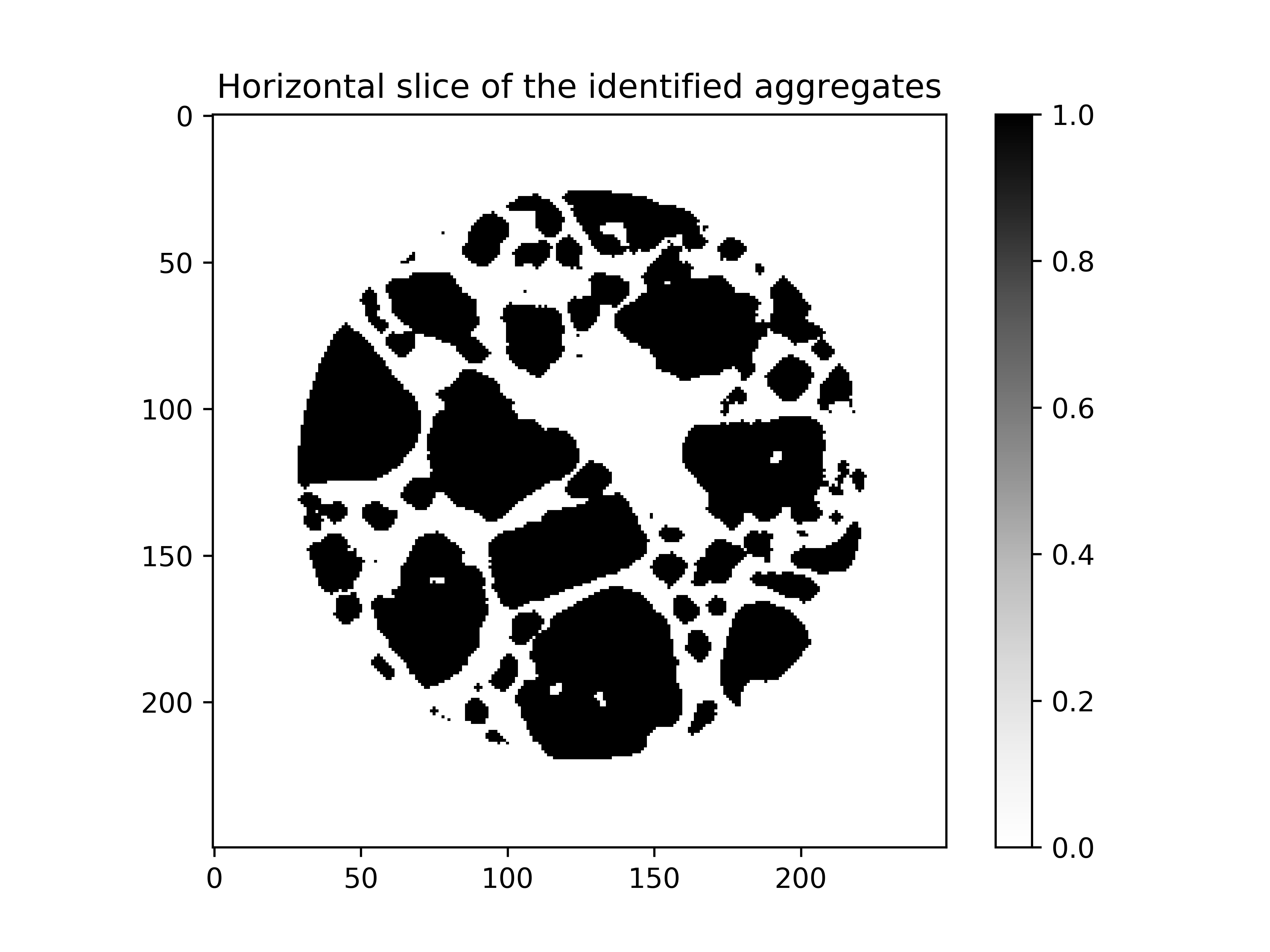
Then the aggregates are dilated 2 times in order to retrieve their original size shrunk by the filter:
# now aggregates are dilated 2 times (could be done with a larger kernel)
aggregates = spam.filters.binaryDilation(aggregates)
aggregates = spam.filters.binaryDilation(aggregates)
plt.imshow(aggregates[aggregates.shape[0] // 2], cmap="Greys")
plt.title("Horizontal slice of the identified aggregates")
plt.show()
Details of the segmentation procedure can be found here: [Stamati2018a].
Step 1.4: Create an array with all the phases identified#
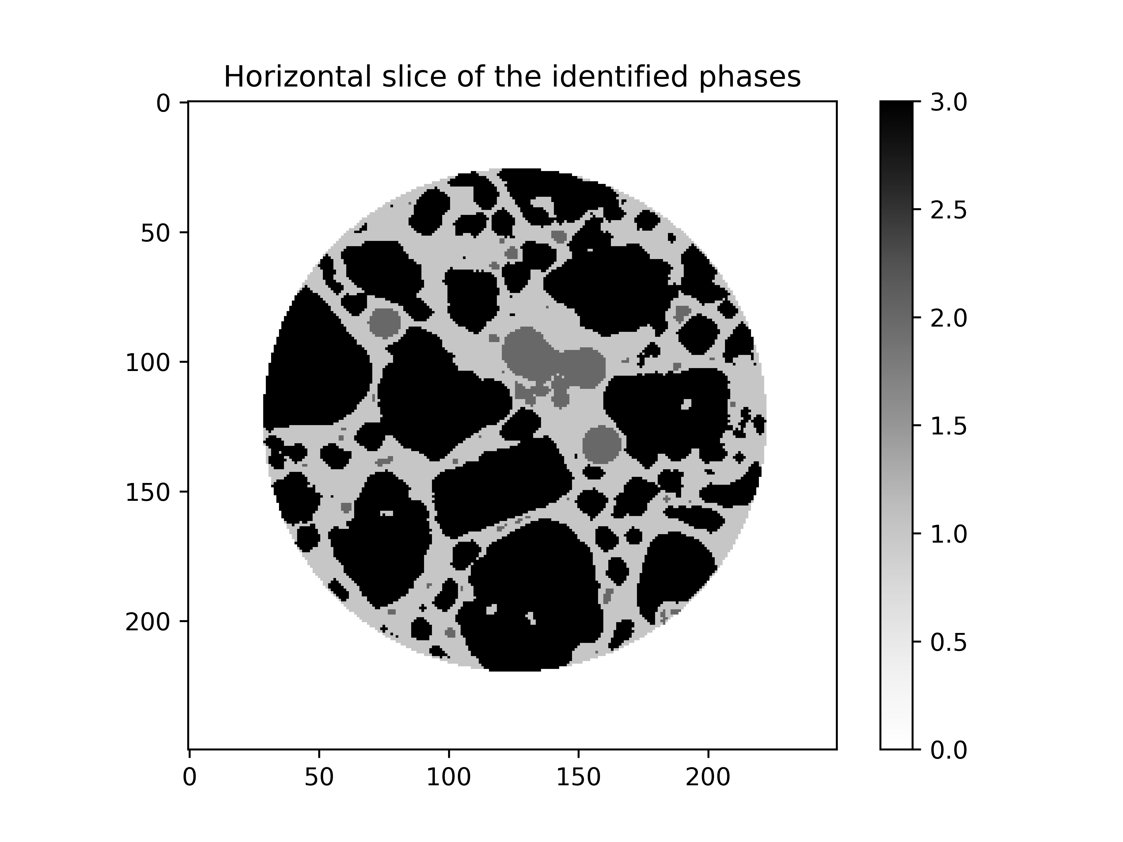
An array with all the phases can now be created where the value of each voxel will represent a phase as:
# outside    -> 0
# mortar     -> 1
# pores      -> 2
# aggregates -> 3
phases = numpy.ones_like(im).astype("<u1") * spam.filters.binaryErosion(mask)
phases[pores == 1] = 2
phases[aggregates == 1] = 3
plt.imshow(phases[phases.shape[0] // 2], cmap="Greys")
plt.colorbar()
plt.title("Horizontal slice of the identified phases")
plt.show()
Step 2: Projection#
Step 2.1: Create the distance fields#
The first step in order to project the phases onto a mesh is to compute a distance field corresponding to each inclusion type phase.
Using this field instead of a raw binary phase field is mandatory since the computation of the interface vector requires a gradient to compute a accurate orientation.
The function mesh.distanceField is used on each inclusion type phase i.e., the pores and the aggregates:
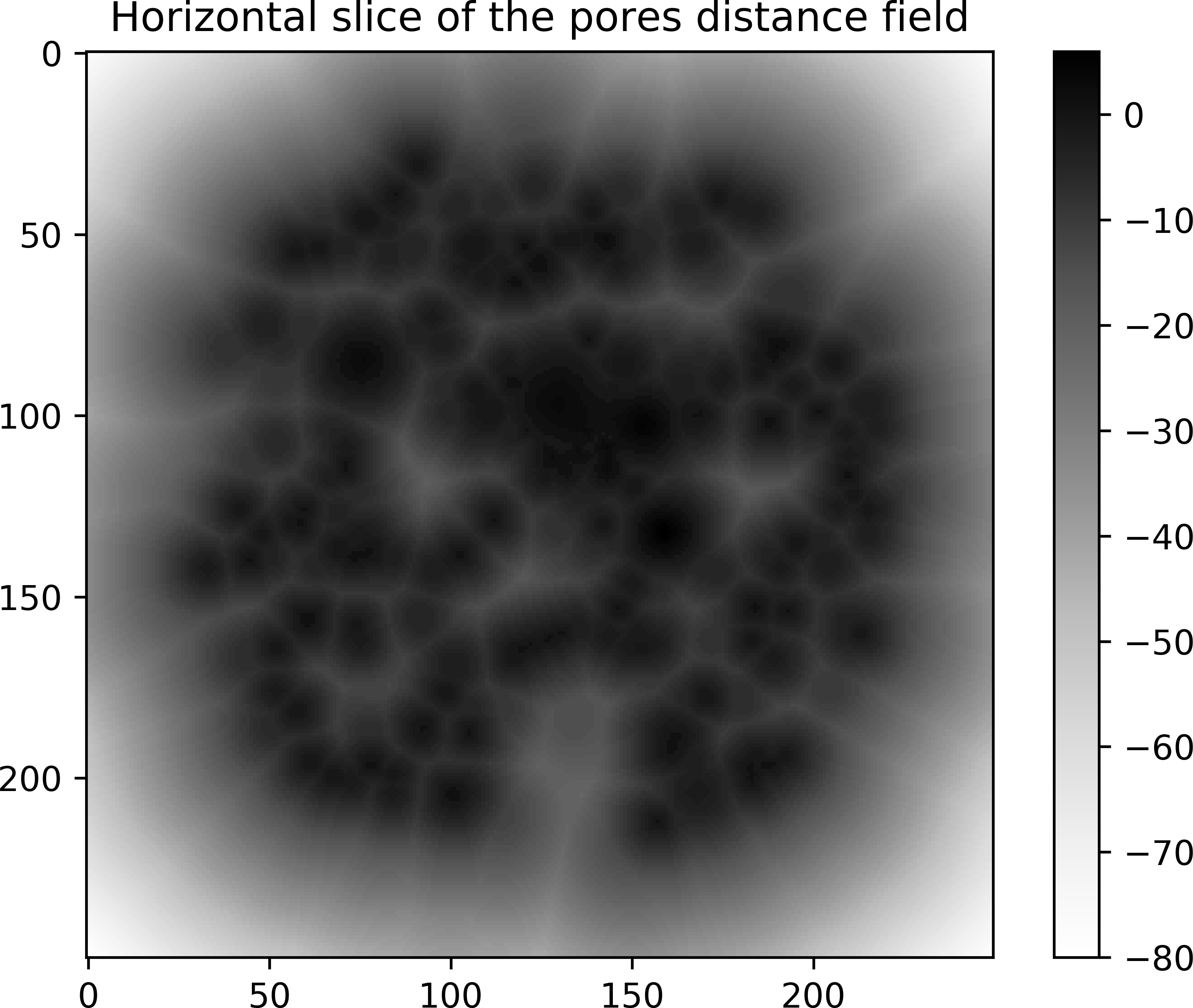
# create the pores distance field (phase value is 2)
poresDist = spam.filters.distanceField(phases, phaseID=2)
plt.imshow(poresDist[poresDist.shape[0] // 2], cmap="Greys")
plt.colorbar()
plt.title("Horizontal slice of the pores distance field")
plt.show()
# Pores distance
# Minimum value: -87.0
# Maximum value: 21.0
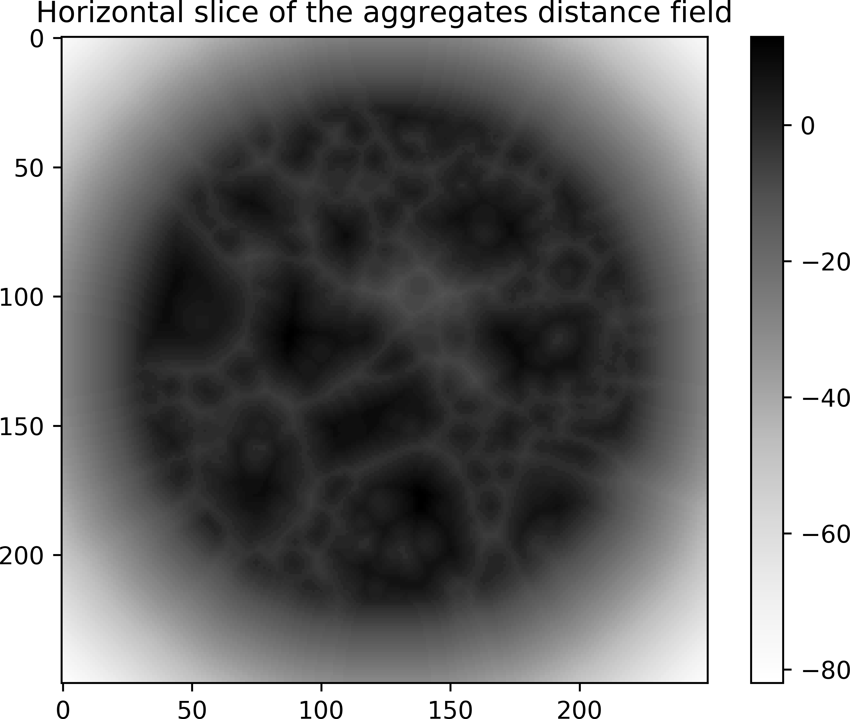
# create the aggregates distance field (phase value is 3)
aggregatesDist = spam.filters.distanceField(phases, phaseID=3)
plt.imshow(aggregatesDist[aggregatesDist.shape[0] // 2], cmap="Greys")
plt.colorbar()
plt.title("Horizontal slice of the aggregates distance field")
plt.show()
# Aggregates distance
# Minimum value: -83.0
# Maximum value: 25.0
We can save now the two fields in a text file that will be needed for the projection. For this step we need to consider the real physical size of the image. Here we have a voxel size of 0.055 mm. We also have to consider the position of the origin of the field in order to coincide with the mesh:
# we save the two fields with the physical sizes of the image
voxelSize = 0.055
width = 0.055 * (phases.shape[1])
fields = {
    "origin": (
        -1.0,
        -0.5 * width,
        -0.5 * width,
    ),  # coordinates of the origin of the field (3 x 1)
    "lengths": voxelSize
    * numpy.array(phases.shape),  # lengths of fields domain of definition  (3 x 1)
    "values": [aggregatesDist, poresDist],  # list of fields
}
For each distance field, the value is positive within the inclusions, negative outside and zero at the interface.
Step 2.2: Create the Finite Element Mesh#
For the projection we need an unstructured 3D mesh made of 4-node tetrahedra. At this stage we have to consider the physical dimensions to the FE mesh. We use the module mesh.unstructured which is a wrapper of meshio to create the needed .msh file and a vtk for visualisation:
# specimen dimensions in mm
centre = (0.0, 0.0)
radius = 5.0
height = 20.0
# characteristic spacing between FE nodes in mm
lcar = 0.2
# create the gmsh file needed for the projection
points, connectivity = spam.mesh.createCylinder(centre, radius, height, lcar)
# create the vtk file (the mesh can be visualised in paraview for exemple)
spam.helpers.writeUnstructuredVTK(points, connectivity, fileName="cylinder.vtk")
# Number of nodes: 124487
# Number of elements: 716525
Step 2.3: Projection#
We can now do the projection from the distance field files (pores and aggregates) and the “void” FE element mesh:
# create dictionnary with mesh data
mesh = {"points": points, "cells": connectivity}
# start the projection
spam.mesh.projectField(
    mesh, fields, writeConnectivity="myFirstProjection", vtkMesh=True
)
The output should look like this:
<projmorpho::set_image
.        field size:     22 x 13.75 x 13.75
.        field origin:   -1 x -6.875 x -6.875
.        field nodes:    400 x 250 x 250 = 25000000
.        field 1
.        .       node 0: -76.3675
.        .       node 1: -76.3675
.        .       [...]
.        .       node 24999998: -77.7817
.        .       node 24999999: -77.7817
.        field 2
.        .       node 0: -83.9166
.        .       node 1: -83.7317
.        .       [...]
.        .       node 24999998: -83.2706
.        .       node 24999999: -83.3607
>
Shift connectivity by 1 to start at 1
<projmorpho::set_mesh
.        number of nodes: 6860
.        number of tetrahedra: 126040/4 = 31510
.        number of midpoints: 189060
>
<projmorpho::compute_field_from_images
.        lengths: 22 x 13.75 x 13.75
.        number of nodes: 400 x 250 x 250
.        number of elements: 399 x 249 x 249
.        field box:
.        .       z = [-1 21]
.        .       y = [-6.875 6.875]
.        .       x = [-6.875 6.875]
.        mesh box:
.        .       z = [0 20]
.        .       y = [-5 5]
.        .       x = [-5 5]
>
<projmorpho::projection
.        field 1 mesh nodes: 6860 mesh mid points: 189060
.        .       MATE,1: background
.        .       MATE,2: phase 1
.        .       MATE,3: interface phase 1 with background
.        field 2 mesh nodes: 6860 mesh mid points: 189060
.        .       MATE,1: background
.        .       MATE,4: phase 2
.        .       MATE,5: interface phase 2 with background
.        Interfaces
.        .      Number of nodes: 77839
.        .      Number of triangles: 14345
.        .      Number of quad: 8701
.        .      Coordinates dim: 3x77839
.        .      Triangles dim: 3x14345
.        .      Quads dim: 4x8701
>
In order to check if the projection went well we can compare the phase repartition on the mesh with the original phase repartition from the previous identification with the VTK files:
myFirstProjection.vtk
myFirstProjection_interfaces.vtk
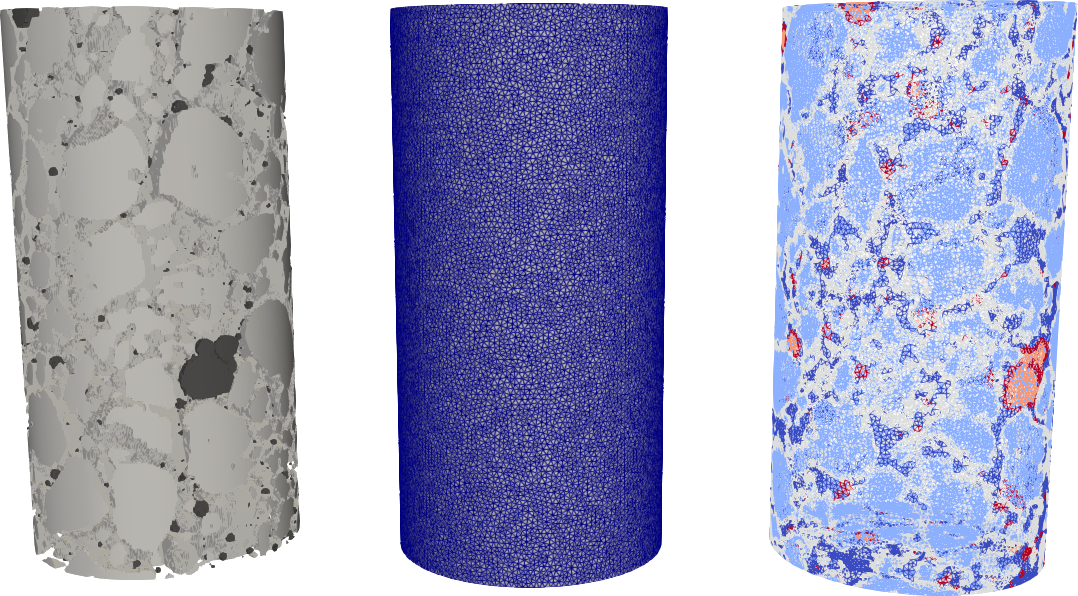
From left to right we see:
1. The phase repartition that comes from the segmentation. We don’t see the voxels since the view is cropped into a cylinder in order to match the mesh size. 2. The finite element mesh. 3. The mesh where every tetrahedron (element) is associated to a phase material (result of the projection).
The pores in black
The aggregates in white
The mortar matrix in grey
These three phases correspond exactly to the right but, in the mesh, there is additional phases (shades of grey) which correspond to elements that have nodes in two different phases (aggregate-matrix and pores-matrix). These elements have several additional information like:
A vector corresponding to the geometrical orientation of the material interface.
A volume corresponding to the subvolume of the inclusion within the element.
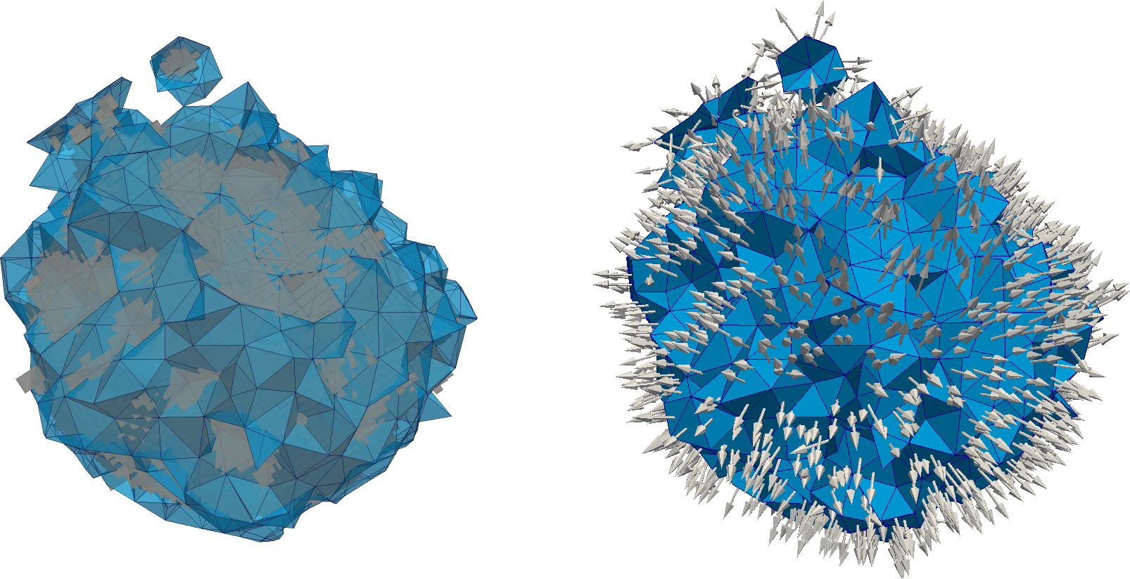
We can see on two figures above a zoom into a single inclusion in the middle of the sample (the matrix has been hidden). On the top it represents a superposition of both the phase repartition that comes from the image (voxels in greys) and only the elements of the mesh with an interface between the matrix and the inclusion (tetrahedra in blue). And below we only show the mesh along with its interface vector mentioned above.
Finally, a mesh file ImyFirstProjection is created that looks like:
COORdinates ! 124487 nodes
1, 0, 0, 0, 0
2, 0, 5, 0, 0
3, 0, 0, 5, 0
4, 0, -5, 0, 0
5, 0, 0, -5, 0
6, 0, 5, 0, 20
7, 0, 0, 0, 20
8, 0, 0, 5, 20
9, 0, -5, 0, 20
10, 0, 0, -5, 20
11, 0, 4.99615, 0.196299, 0
12, 0, 4.98459, 0.392295, 0
13, 0, 4.96534, 0.587687, 0
[...]

ELEMents ! 716525 elements
1, 0, 4, 40134, 82981, 61631, 113664, 0, 1, 0, 0
2, 0, 1, 34761, 66609, 60357, 82884, 0, 1, 0, 0
3, 0, 3, 39371, 50046, 8289, 64659, 0.00116549, 0.878333, 0.477637, 0.019834
4, 0, 2, 24061, 39160, 49569, 67152, 0, 1, 0, 0
5, 0, 2, 37050, 59636, 22794, 61616, 0, 1, 0, 0
6, 0, 2, 23838, 64198, 60690, 71504, 0, 1, 0, 0
7, 0, 3, 42354, 49334, 32016, 85847, 0.00030443, -0.756086, -0.501135, 0.420948
8, 0, 3, 44408, 47029, 26307, 72025, 0.000427038, -0.576798, 0.401879, -0.711195
9, 0, 3, 42694, 42798, 26651, 100327, 0.000951016, 0.491136, 0.211643, -0.844981
10, 0, 3, 27264, 51682, 41300, 66979, 6.25952e-05, 0.872644, 0.449371, 0.191201
11, 0, 3, 39594, 36201, 75550, 84799, 0.00127971, -0.0692717, -0.120987, 0.990234
12, 0, 3, 98525, 112643, 59425, 118182, 5.50818e-05, 0.103265, 0.837309, -0.53689
13, 0, 3, 30964, 54757, 35809, 56465, 0.000117003, -0.667076, 0.397527, 0.630065
14, 0, 3, 56470, 81354, 58111, 86734, 0.00106211, 0.720656, 0.500064, -0.480198
15, 0, 3, 25043, 54420, 49697, 79081, 0.00108912, -0.644494, 0.661685, 0.383145
16, 0, 5, 24150, 95380, 70448, 113407, 7.73197e-08, 0.657214, -0.0430983, 0.752471
17, 0, 2, 36712, 74936, 69373, 107451, 0, 1, 0, 0
[...]
where the COORdinates list corresponds to the node positions:
nodeNumber, 0, x, y, z
and the ELEments list coorresponds to the connectivity matrix + interfaces information:
elementNumber, 0, phaseNumber, node1, node2, node3, node4, subVolume, interfaceVectorX, interfaceVectorY, interfaceVectorZ
Note that by default, if no geometrical interface is given for an element, the subvolume is 0 and interface vector is [1, 0, 0].
Conclusion#
It’s groovy!
References#
Roubin, Emmanuel, et al. “Multi-scale failure of heterogeneous materials: A double kinematics enhancement for Embedded Finite Element Method.” International Journal of Solids and Structures 52 (2015): 180-196. https://doi.org/10.1016/j.ijsolstr.2014.10.001
Stamati, O., Roubin, E., And, E. et Malecot, Y. (2018). Phase segmentation of concrete x-ray tomographic images at meso-scale: Validation with neutron tomography. Cement and Concrete Composites, 88:8 – 16. https://doi.org/10.1016/j.cemconcomp.2017.12.011
Stamati, O., Roubin, E., Andò, E., & Malecot, Y. (2018). Tensile failure of micro-concrete: from mechanical tests to FE meso-model with the help of X-ray tomography. Meccanica, 1-16. https://doi.org/10.1007/s11012-018-0917-0