Do you have images of the same object acquired with different techniques (e.g., x-ray, neutron, MRI)?
Here we will learn to align them in order to then be able to analyse them together: this can greatly help with segmenting phases, or doing a coupled analysis as, for example, in [Stavropoulou2020], [Robuschi2021], [Tornquist2021], [Sleiman2022].
Multimodal registration (MMR) can be seen as a generalisation of the classical registration process (described in tutorial Tutorial: Image correlation – Practice) applied to fields of the same material and coordinate system, but acquired with different modalities (i.e., with complementary attenuation sensitivities to the material phases).
We will be using the Multimodal Registration Technique whose mathematical foundations are proposed in [Tudisco2017] and implemented in [Roubin2019], this technique is an improvement over the more classic mutual information techniques because it takes into account the noise and uncertainty on phase identification. These two papers are excellent references should you have any doubt about the underlying reasons for the operations performed in this tutorial.
The final output of this process will be a pair of aligned images, and a phase map which can be of interest by itself. This example tutorial will focus on field images acquired using two modalities from x-ray and neutron tomography, but any two images can be used.
In this tutorial we will use the SandNX.zip dataset spam tutorial archive on zenodo, a dataset consisting of an X-ray tomography and a neutron tomography scan of a partially saturated sand, kindly contributed by Marius Milatz in Hamburg University and acquired at the NeXT Neutron and X-ray Tomography instrument [Tengattini2020] at the ILL in Grenoble.
We recommend you take a piece of paper and pen, open up your two volumes, and write a table of the approximate greyvalue for each (main) phase you can see in your image.
For the data above, here’s a very rough guess:
Rough measurement of the CT-value of the phases present in the image
The fundamental concept on which the technique is based is the Joint Histogram.
This is a histogram computed based on two images, where pairs of voxels at the same position in both images are binned into a 2D space.
The joint histogram therefore has a total number of counts equal to the pixels of one of the two images.
The figure below illustrates the joint histogram for well-aligned slices, with three peaks present, which correspond well to the three phases identified by hand above.
Illustration of the joint histogram for a since aligned slice for this dataset
This is the final result we’re seeking, but most likely when you start the process, before aligning the images, your bivariate histogram will look a bit like this:
Illustration of the joint histogram for a still misaligned slice for this dataset
In this case the X-ray CT values corresponding to the grains (around 33500 counts) correspond to a variety of values in the neutron image (from ~18000 to ~40000) , as highlighted by the long horizontal streak. This is because to a grain in the x-ray image different phases appear in the misaligned neutron image, for example.
The final purpose is to create a dictionary matching correctly neutron and x-ray values. We will fit on each peak a bivariate gaussian distribution (that is, a gaussian with two axes, corresponding to the x-ray and neutron axes). This will be a key step in the registration, as it will allow us to speed up the alignment optimisation detailed in section Phase map and multimodal registration.
Before starting with your own data, you need to make sure that the two 3D volumes that you want to register have the same number of pixels and are roughly (+-20%) the same size. If the former is not the case, the smaller image should be padded to match the size of the larger image. If the latter condition is not respected, you should consider scaling up or down one of the two images.
The original, unbinned images will likely be rather large and contain a lot of details. It is generally convenient to start an initial registration with a heavily binned (4 or more) dataset, get a first, quick, alignment, which will converge faster and more easily allow for larger displacements (because of the larger “size” of a pixel) followed by a repetition of the operation at lower binning levels, as in a pyramid (and similarly to what is done in same-type image registration in this tutorial).
The result of the first alignment can be directly used as an input for the following steps, the software will understand different binning levels and automatically adjust for it, so it is convenient to save the two datasets at different binning levels before starting.
Another choice to make is which image will be deformed/moved. As in all transformations this will entice an interpolation of the dataset and therefore a certain loss of sharpness. In this case it is Image 2 which will be deformed. Furthermore the registration algorithm is full-newton so the gradient calculation will be performed on the deforming image. The choice of which image to put as first is therefore entirely problem dependent. If in doubt, you can try both! In this tutorial we use the neutron tomography as Im1 and the x-ray tomography as Im2.
The multimodal registration suite comprises a graphical user interface, which allows for an user-driven eye pre-alignement, followed by a peak fitting of the bivariate histogram, followed by the automated image registration. There is also a command line script (spam-mmr) which only covers the last two steps.
Within the spam virtual environment the graphical user interface can be launched using the following command:
(spam)$ spam-mmr-graphical\ # the script $ im1.tifim2.tif\ # the two 3D images (tiff files) to correlate [necessary] $ phi.tsv\ # Any pre-existing transformation tensor [optional] $ Crop.tsv# Any pre-exisiting cropping of the image. [optional]
You should end up in the welcome screen in the figure below, which should look something like this:
Welcome Screen of the Graphical User Interface. Make sure to select the correct binning level of the images loaded with the script or that will be loaded in the next step. This will allow spam-mmr-graphical to translate the meaning of the transformation and cropping matrices across different binning levels.
Please note that launching directly spam-mmr-graphical without the other arguments also works and will prompt you to manually select the two images as well as the transformation tensor and cropping (after clicking the “next step (eye registration)” button on the welcome screen). If you don’t have the latter two, simply press cancel when prompted.
When ready, press the “Next step (Eye Registration)”. You should get to the visual alignment screen:
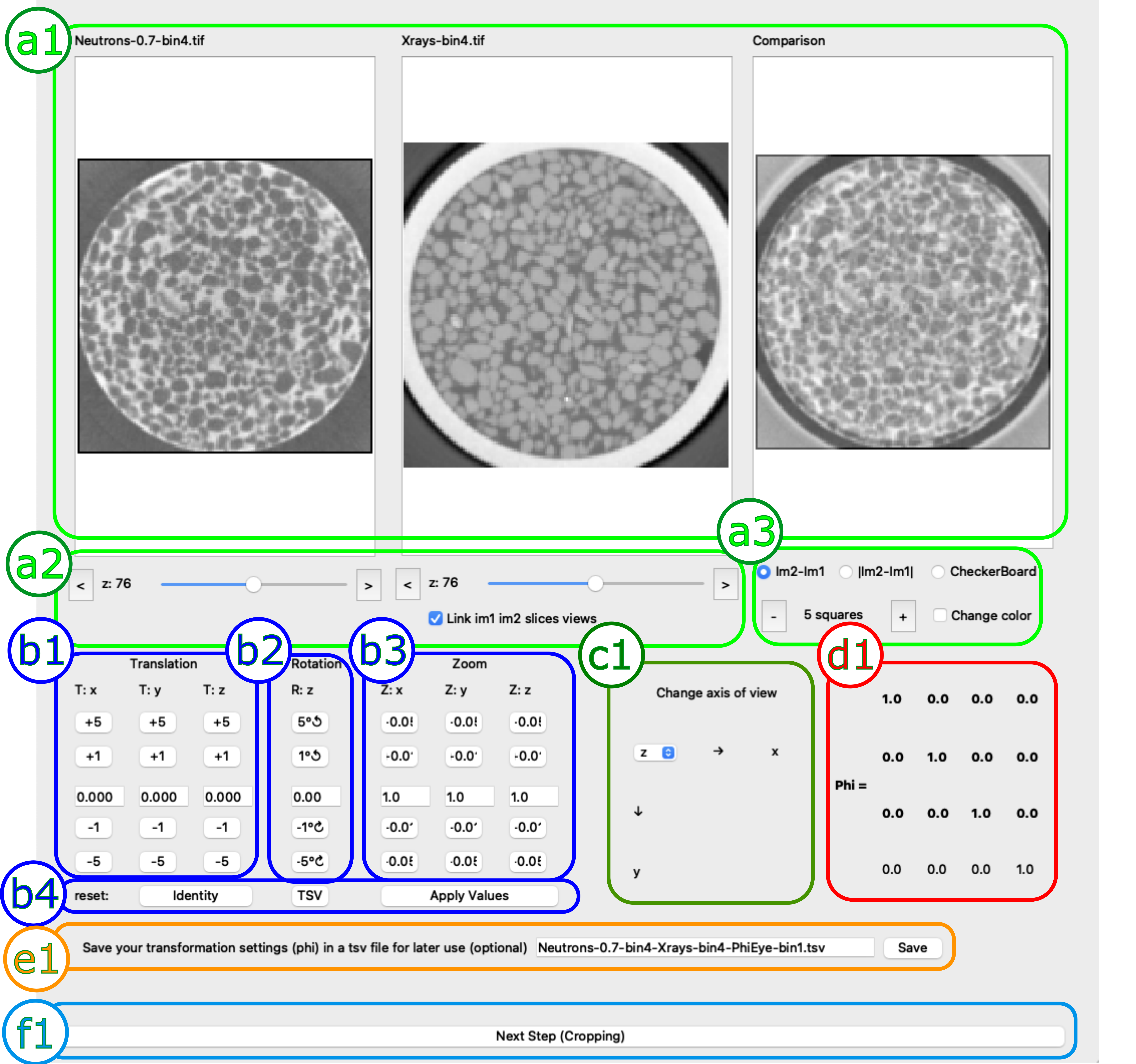
Visual Alignment Scheme, divided here in 6 submenus
Note
Submenu a: “visualisation”
a1: slice of image 1 (left), image 2 (centre) as well as their comparison (right):
a2: selected slice in image 1 (left), image 2 (centre). These two are, by default, linked. This connection can be removed by un-checking the “Link im1 im2 slice views” button, after which the two slices can be moved individually. A new button will appear that will allow to add a vertical shift between the two (∆z= xx) and re-link the two bars. This will change the z value in submenu b1
a3: controls for the comparison slice, which can be the difference between the two images, its norm or a checkerboard (with its dedicated buttons to adjust the number of subdivisions in the checkerboard ad to change their colours)
Submenu b: “alignement”
b1: Translation of the slice in the x, y and z directions the buttons will add + or - 1 or 5 voxels, respectively. The textboxes will give the absolute values which can be changed by any amount (even sub-pixels). Please note that the values in these boxes are absolute. Please also note that to take these values into account you must click on “Apply Values” (submenu b4)
b2: Rotation; analogous to the previous one but rotation adjustment. Please note that in this case the textboxes will provide the relative value
b3: Zoom; adjusts the zoom, works analogously to the previous ones
b4: Control of the boxes; the “identity” button resets the transformation to an identity matrix (no translation, rotation, zoom), the “TSV” button loads the values saved in the TSV savefile pointed to in the submenu e1. The “Apply values” button applies the values in the textboxes in menus b1, b2 and b3. Please note that Translation and Zoom will take them as absolute values, while rotation will consider the value there as relative
Submenu c: “reslice”:
c1: decides along which plane the volume is resliced. For example in the figure above it’s an horizontal slice (z) of the vertically oriented, cylindrical sample. The menu also reports with arrows the positive direction of the movement.
Submenu d: “transformation matrix”
d1 this the transformation matrix Phi, it is simply the result of the operators in submenu b. If it’s not saved a highlighted “Phi needs to be saved” reminder will be displayed.
Submenu e: saving
e1 Indicates the path where the transformation matrix in submenu d1 is saved, for later use.
Submenu f: next
f1: by clicking this button you jump on the cropping menu.
In this case, the initial alignment is simply an identity matrix because we did not have any prior information. Some steps that can be used for this specific dataset to pre-align the images are:
Z-adjustment: Unlink the two images (Checkbox in submenu a2), and move image two up by 5 slices: relink them by clicking “Apply ∆z=5”. For this vertical alignment phase, you can often use the bottom of the sample as a reference (if contained within the image), so for example z=139 corresponds roughly to z=144 of the second image (X-ray in this case).
We also immediately notice that there is a rotation of 180˚ in the image. Please note that if you notice that if the images are “flipped” along any axis this cannot be corrected within the software (for how the transformation matrix is defined here), and should be done externally and then the correctly flipped images should be used for the following steps (for all binning levels!). Rotate the image by 180˚ (Submenu b2). Note that every applied rotation is relative to the previous one and not an absolute rotation from the initial image position (unlike the translation)
Dezoom the second image until 0.95. Please note that, while the software allows to stretch the image in all directions independently, often the magnification correction is isotropic (al least in neutron/x-ray volumes) In this operation, the boundaries (e.g., of the cells or of the sample) can be very helpful for alignment.
here we notice that because we modified the z-scaling the two images are not aligned vertically anymore, This is an iterative process after all! We then move the second image down by another 3 pixels (z=139 corresponds to z=147).
Now the images look coarsely aligned; save this visual approximation (Submenu e1) which serves as an initial guess for the next step: cropping
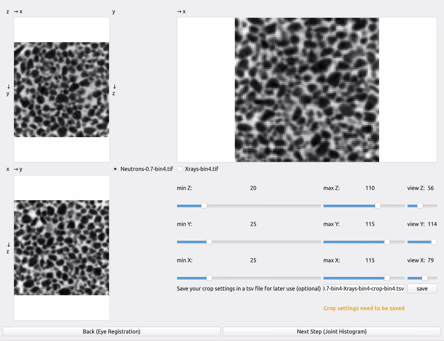
Image cropping menu: it allows to crop the outside of the figure and remove less-than-useful bits. Please note that air surrounding the sample can hinder the convergence of the algorithm.
This menu allows for cropping the image, please note that homogeneous regions (e.g., air around the sample) does not help guide the mmr optimisation, so, should ideally be removed and so as to only keep regions with good contrast. As shown in the figure above, sliders can be used to crop the left and the right parts of the image (left and centre sliders, respectively), for each axis. The right hand slider allows you to choose different visualisation slices. Please note that while you can directly continue to the next menu (Joint Histogram) it is recommended to save (the software proposes a saving file/location but it can be changed) the cropping matrix for re-use in following steps (e.g., at lower levels of binning, or future reference).
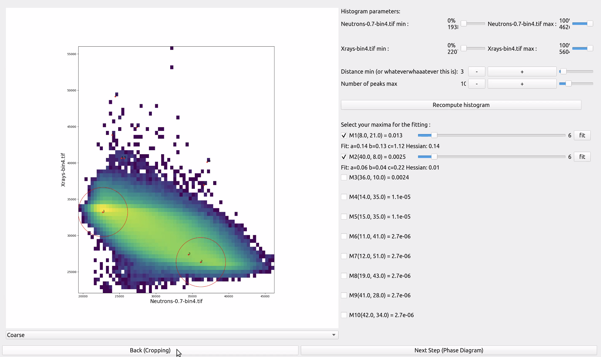
Joint Histograms Menu, which allows you to select the peaks of the bivariate histograms and their parameters
The software now computes the Joint Histogram (introduced in Section Introducing the Joint Histogram) of the two pre-aligned images. The following step consists in fitting nice smooth surfaces (bivariate gaussians) to this data. The software automatically calculates some peaks/local maxima around which to centre these surfaces, but it proposes more peaks than you may need, and some peaks might be spurious (caused by bad pre-alignment) or some neighbouring peaks may just be one phase, but because of local minima they may appear as multiple peaks. You must then choose peaks that “make sense” for your specific images, and where possible, look for peaks corresponding to the phases you identified before (section Before you start). The software also allows you to adjust the radius around which to fit these curves with the horizontal slider. It defaults to 6 but some phases might have narrower distributions (less variations in the pixel values for that phase) or larger ones. If you modify this value make sure to click on the “fit” button to relaunch the bivariate gaussian fitter.
Three coefficients describing the bivariate Gaussian are computed by the fitting algorithm, corresponding to the variances in the two cardinal axes (a and c) and proportional to the product of the standard deviations in the two cardinal axes. The Hessian of this matrix of coefficients is also computed, as it provides a useful sanity check, since maxima should have a positive Hessian while saddle points will have a negative one, for example. More details about the mathematical foundations of this operation can be found at [Roubin2019] .
In the figure above we identify two peaks (peaks 1 and 2). Based on their grayvalues, we deduce that they belong to grain and water phases, respectively. Please note that you do not need for the first iterations to recognise all the different phases, and more can be added at lower, richer, binning levels (as detailed in section Preparing the data).
Sometimes there are spurious peaks at very high (e.g., saturation) or very low (e.g., air around the sample) attenuation values of the histogram that you may want to exclude from the following steps.
The software then allows you to recompute the whole histogram in between different minimum and maximum values (top part of the menu both as percent and as absolute value limits). Similarly, if you have too many cases of distinct peaks close by that are just one larger phase, you can increase the minimum distance between local maxima that the software will consider as individual peaks, and increase or decrease the total number of identified peaks (second and third line in the menu to the right). Remember to click on ‘Recompute histograms’ if you modify any of these parameters.
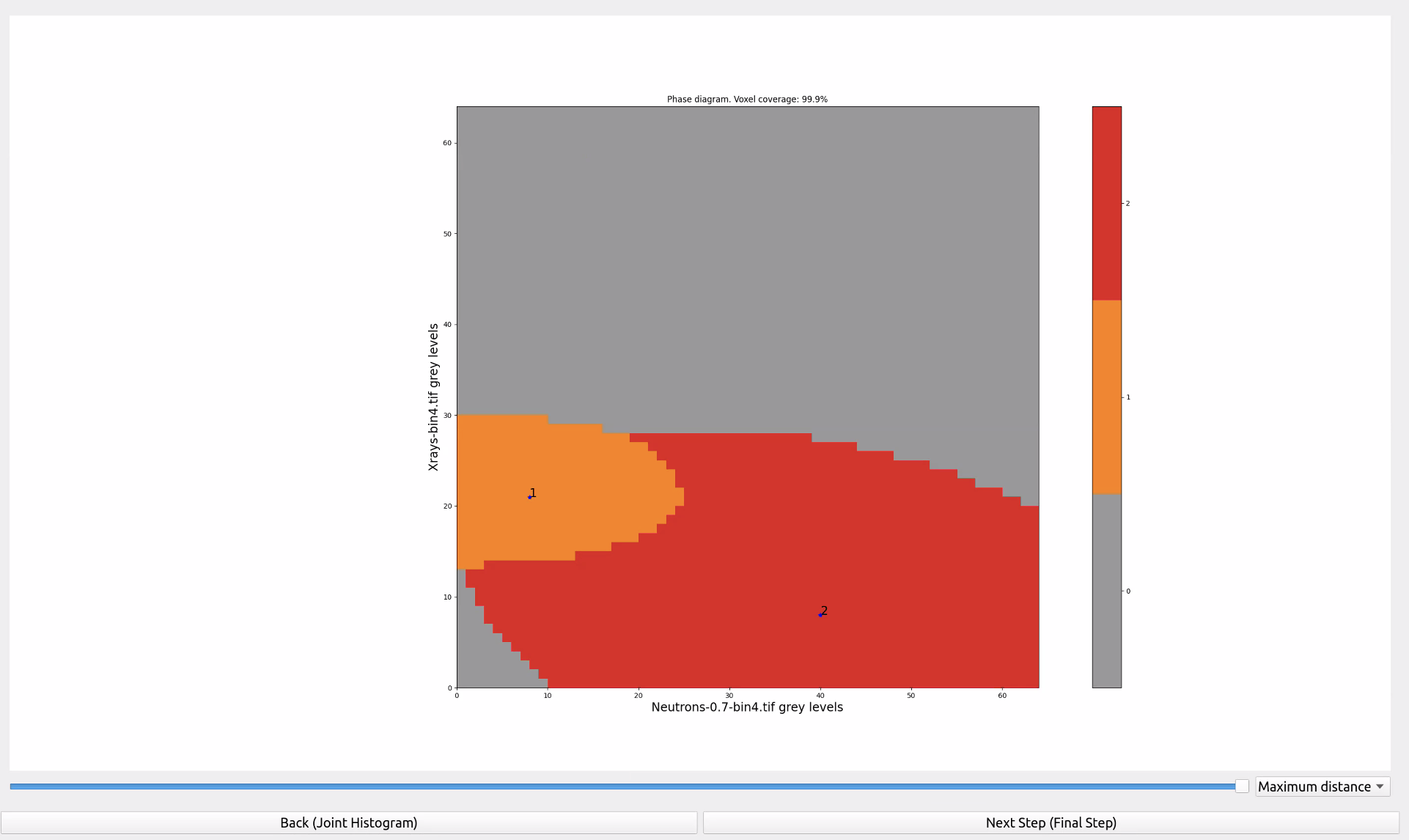
In this menu the software recomputes the histogram based on 64x64 bins and shows all the phases comprising the joint histogram. Using one one colour per phase it highlights how much of the histogram is considered as covered by the bivariate gaussian curves representing each phase. If you think that one of these surfaces is talking too much space (e.g., invading areas you’re sure to belong to another phase you decided to ignore at this stage) you can reduce the overall coverage of the space. Different approaches can be used to determine how much to reduce them (based either on the maximum distance or the Mahalanobis one, see [Roubin2019], section 2.4 for more details).
The next step is the phase diagram of the image, i.e., an image where all the phases have been identified and assigned the colours just determined in the phase diagram. The more you have reduced the coverage in that step, the more unassigned voxels you will see. You can go back and forth between this screen and the previous one to change the coverage if the expected phases are poorly segmented.
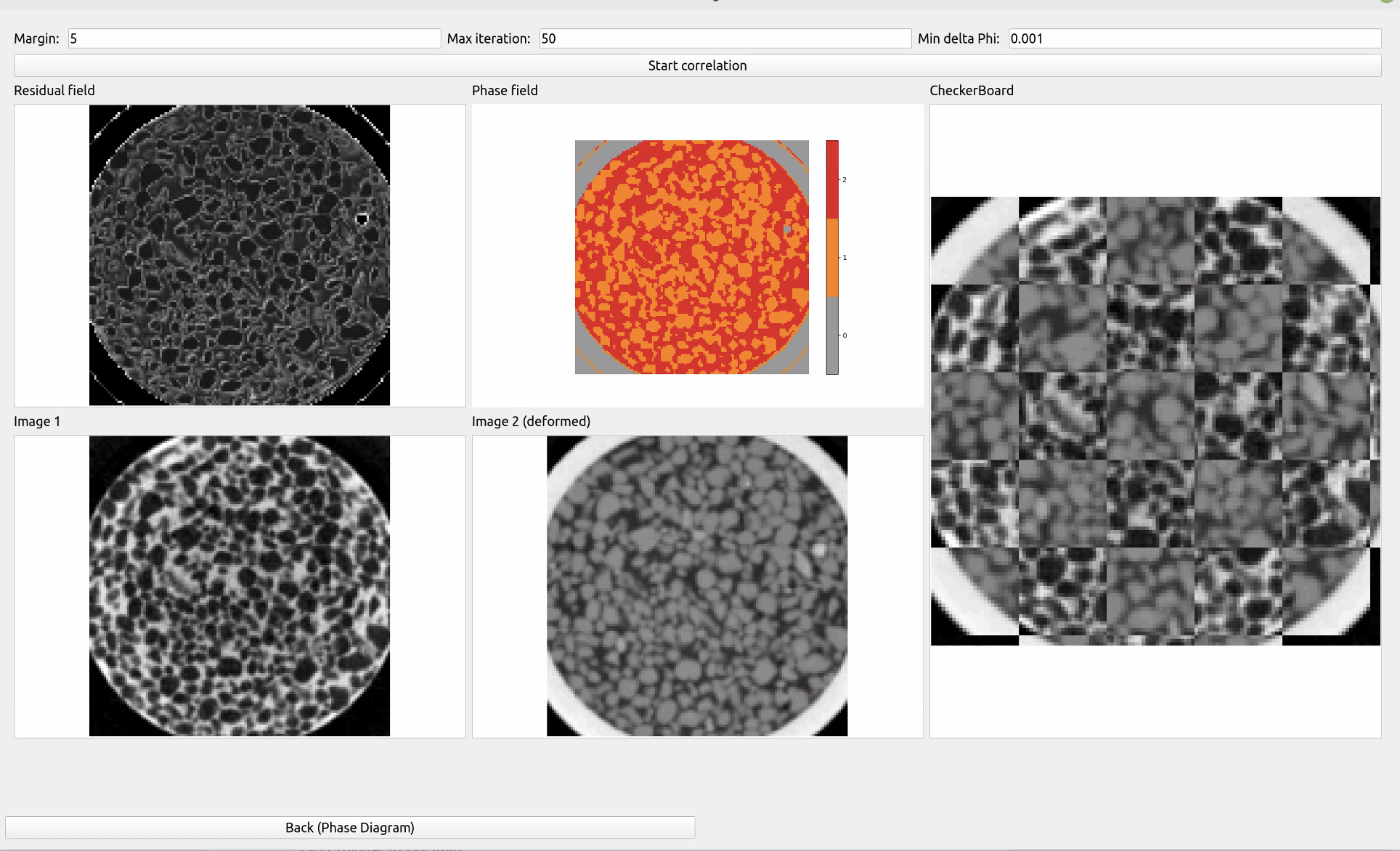
This is the last step, in which the software actually does the automated alignment. Please note that the script spam-mmr starts essentially from this point and the aforementioned guided steps need to be performed directly and passed to the script.
When you click on “start correlation”, the software will automatically move im2 to align the images by minimising the residual. The menus show you the residual field (i.e., the “error” in alignment, which we are trying to minimise), the phase field (i.e., the pre-segmented image where the different composing phases are identified on a given slice) as well as the original im1 and im2 and their checkerboard composition.
Generally it should find an optimum before the default number of steps is reached, but you can increase their number in the top menu. You can also modify the convergence criterion “Min delta Phi” (the smallest variation in correlation value measured over a given step; its reduction being symptomatic that the software found a stable maximum). In the top menu you can also control how many pixels on the margin of the deforming image to ignore.
At the end of this step the software automatically saves the updated deformation matrix as well as the aligned volumes and the segmented image (i.e., an image where the phases are identified) in the same folder as the original image. If this step did not work, you can move back and forth across the menus with the arrows at the bottom of the page until you find the best set of parameters for the software to perform this registration step.
If you have started, as suggested at the beginning of the tutorial, at a high binning level (e.g., 4) you can now move to a lower binning level (e.g., 2 and then 1) so as to further refine the alignment. All the pre-alignment information saved at the end of this step can be automatically reused for the lower binning levels.
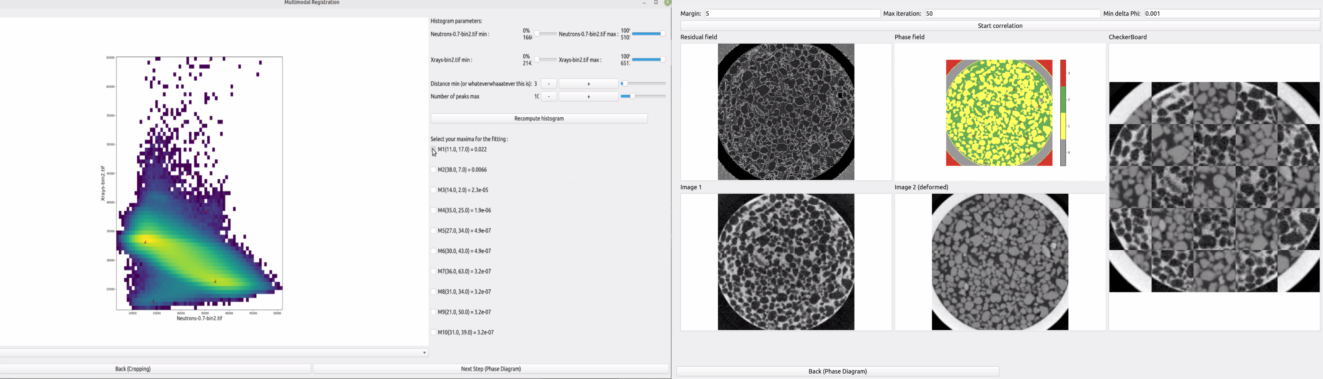
Menus when re-running the MMR-graphical script at a lower bining level
Open spam-mmr-graphical, and input images at a different binning level as detailed in Section Preparing the data. Make sure to select the right binning level in the start screen, and to maintain im1 and im2 the same modalities (im1= neutron and im2= X-rays, here).
You can now also load the cropping and alignment matrices computed in the previous steps at higher binning levels. If you had correctly selected the binning level at the beginning of the previous steps they should be saved as “yourFileName-crop-binXX” and “yourFileName-PhiFinal-binXX”, where XX is the beginning level and the software will automatically adjust the alignment and cropping to match to the current binning level.
In principle the eye registration and the cropping steps should be straightforward as the images are already pre-aligned.
The following steps are also analogous to the iteration detailed above, but the joint histogram should look a bit “richer” now (see figure above), with more peaks and smoother curves. If your object had more phases than identified at lower binning levels (e.g. pores that were invisible at higher binning levels) it is now a good time to add them to the list of the fitted bivariate gaussian curves. In the last menu, start the correlation again, you will notice that this time the process is slower now (bigger images!). Once this is done at this binning level, you can go to the one above (if any are left)!
You now have a transformation and a cropping matrix that you can directly apply with spam.deformation.computePhi (see dedicated tutorial: Tutorial: Image correlation – Practice) as well as a pre-deformed image 2 at the current binning level!
Stavropoulou, Eleni, Edward Andò, Emmanuel Roubin, Nicolas Lenoir, Alessandro Tengattini, Matthieu Briffaut, and Pierre Bésuelle. Dynamics of water absorption in Callovo-Oxfordian claystone revealed with multimodal x-ray and neutron tomography. Frontiers in Earth Science 8 (2020): 6. https://doi.org/10.3389/feart.2020.00006
Robuschi, Samanta, Alessandro Tengattini, Jelke Dijkstra, Ignasi Fernandez, and Karin Lundgren. A closer look at corrosion of steel reinforcement bars in concrete using 3D neutron and X-ray computed tomography. Cement and Concrete Research 144 (2021): . https://doi.org/10.1016/j.cemconres.2021.106439
Törnquist, Elin, Sophie Le Cann, Erika Tudisco, Alessandro Tengattini, Edward Andò, Nicolas Lenoir, Johan Hektor et al. Dual modality neutron and x-ray tomography for enhanced image analysis of the bone-metal interface. Physics in Medicine & Biology 66, no. 13 (2021): https://doi.org/10.1088/1361-6560/ac02d4
Sleiman, Hani Cheikh, Alessandro Tengattini, Matthieu Briffaut, Bruno Huet, and Stefano Dal Pont. Simultaneous x-ray and neutron 4D tomographic study of drying-driven hydro-mechanical behavior of cement-based materials at moderate temperatures. Cement and Concrete Research 147 (2021): 106503. https://doi.org/10.1016/j.cemconres.2021.106503
Tengattini, Alessandro, Nicolas Lenoir, Edward Andò, Benjamin Giroud, Duncan Atkins, Jerome Beaucour, and Gioacchino Viggiani. NeXT-Grenoble, the Neutron and X-ray tomograph in Grenoble. Nuclear Instruments and Methods in Physics Research Section A: Accelerators, Spectrometers, Detectors and Associated Equipment 968 (2020): 163939. https://doi.org/10.1016/j.nima.2020.163939
Roubin, Emmanuel, Edward Ando, and Stéphane Roux. The colours of concrete as seen by X-rays and neutrons. Cement and Concrete Composites 104 (2019): 103336. https://doi.org/10.1016/j.cemconcomp.2019.103336
Tudisco, Erika, Clément Jailin, Arturo Mendoza, Alessandro Tengattini, E. Andò, Stephen A. Hall, Gioacchino Viggiani, Francois Hild, and Stéphane Roux. An extension of digital volume correlation for multimodality image registration. Measurement Science and Technology 28, no. 9 (2017): 095401. https://doi.org/10.1088/1361-6501/aa7b48