Fix segmentation issues

This example shows how to use the function to detect and fix under and oversegmentation

import matplotlib
import matplotlib.pyplot as plt
import numpy
import spam.kalisphera
import spam.label

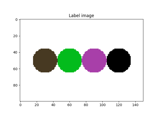
Create label image

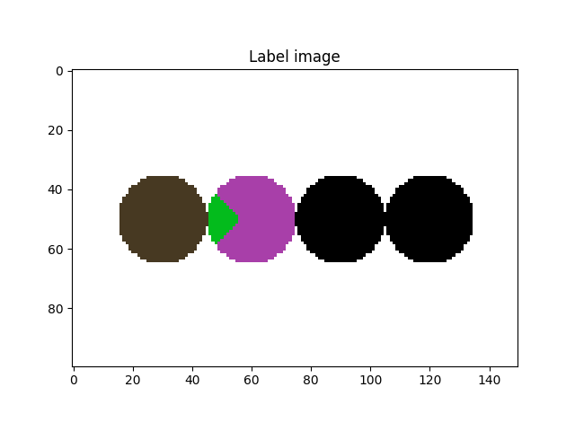
Let’s create a label image that has both problems: oversegmentation (one grain is labelled as two different grains), and undersegmentation (two grains are labelled as one grain).

# First create a seed image, this will be used to induce the segmentation problems
seeds = spam.kalisphera.kalisphera.makeBlurryNoisySphere(
    (100, 100, 150),
    [[50, 50, 30], [50, 50, 50], [50, 50, 60], [50, 50, 90]],
    [15, 5, 5, 15],
)
# Label the seeds
imSeedLab = spam.label.watershed(seeds > 0.5)
# Create the binary of the "true" particles
imGrey = spam.kalisphera.kalisphera.makeBlurryNoisySphere(
    (100, 100, 150),
    [[50, 50, 30], [50, 50, 60], [50, 50, 90], [50, 50, 120]],
    [15, 15, 15, 15],
)
# Labels the image and use the seeds, since there is an offset between the seeds and the true image, we will have segmentation problems
imLabel = spam.label.watershed(imGrey > 0.5, markers=imSeedLab)
# Let's take a look at it
fig = plt.figure()
plt.subplot(1, 1, 1)
plt.gca().set_title("Label image")
plt.imshow(imLabel[50, :, :], cmap=spam.label.randomCmap)
plt.show()

Undersegmentation

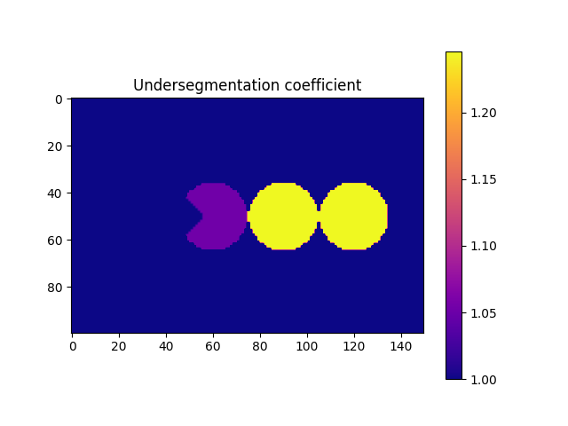
Let’s start by dealing with the undersegmentation of the particles on the right side of the previous image (label # 4)

# First compute the undersegmentation coefficients
underSegCoeff = spam.label.detectUnderSegmentation(imLabel)
# Colour the label image with the coefficients
imUnderSeg = spam.label.convertLabelToFloat(imLabel, underSegCoeff)
# Let's plot them and see what do they look like
fig = plt.figure()
plt.subplot(1, 1, 1)
plt.gca().set_title("Undersegmentation coefficient")
plt.imshow(
    imUnderSeg[50, :, :],
    cmap=matplotlib.pyplot.cm.plasma,
    vmin=1,
    vmax=numpy.max(underSegCoeff),
)
plt.colorbar()
plt.show()

|                                                             | ETA:  --:--:--
|###############                                               | ETA:  0:00:00
|###############################                               | ETA:  0:00:00
|##############################################                | ETA:  0:00:00
|##############################################################| ETA:  0:00:00
|##############################################################| Time: 0:00:00

The function compute the convex volume of each particle and compares it against its own volume. In priciple, all particles should have a value of 1, however there is a small tolerance given

the discretization of our system. We now need to generate a list of target particles that we want to fix. In this example, we are going to use a value of 1.2, taken directly from the previous figure. However, when particles are not homogenous in size/shape (as 99% of the materials we scan) we should take a look at the distribution of the coefficients. A “safe” approach is to select the

threshold as : math:mu +4* \(\sigma\), where \(\mu\) and \(\sigma\) are the mean and standard deviation of the distribution of coefficients.

targetUnder = numpy.where(underSegCoeff > 1.2)[0]

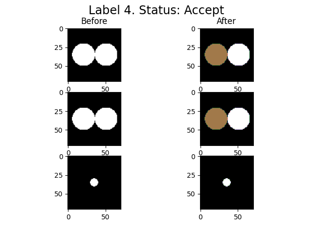
With the list of target particles at hand, it is time to fix it. The function performs a segmentation at a higher threshold over the subset of the particle, in order to try to split the selected particles. For this, we need to feed the greyscale image as well. It is important to note that the greyscale must present a normalised histogram (please refer to the example

corresponding to Histogram normalisation).

imLabel2 = spam.label.fixUndersegmentation(imLabel, imGrey, targetUnder, underSegCoeff, imShowProgress=True, verbose=True)

|                                                             | ETA:  --:--:--
|##############################################################| ETA:  0:00:00
|##############################################################| Time: 0:00:00

spam.label.fixUndersegmentation(): From 1 target labels, 1 were modified

We activated the imShowProgress key, so we can see (label by label) the result of the function. Given the simplicity of the data, the function was able to separate the two particles. However, depending on the morphology of the grains and the quality of the greyscale image, there might be some cases where the function is not able to separate the grains. Let’s take a look at the current state of the label image.

fig = plt.figure()
plt.subplot(1, 1, 1)
plt.gca().set_title("Label image")
plt.imshow(imLabel2[50, :, :])
plt.show()

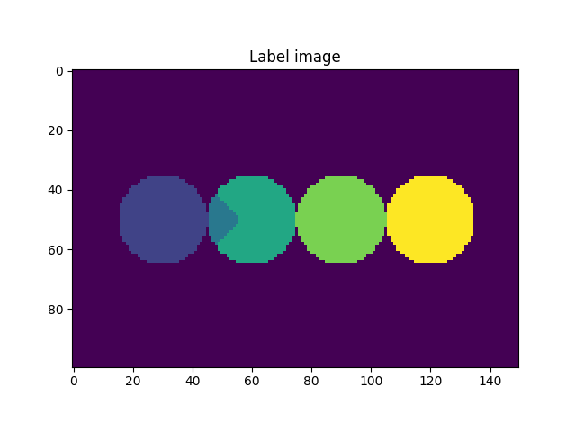
Oversegmentation

# From the previous image we saw that we still need to deal with the oversegmentation. First let's compute the oversegmentation coefficient, and colour each label accordingly.

overSegCoeff, touchingLabels = spam.label.detectOverSegmentation(imLabel2)
imOverSeg = spam.label.convertLabelToFloat(imLabel2, overSegCoeff)
fig = plt.figure()
plt.subplot(1, 1, 1)
plt.gca().set_title("Oversegmentation coefficient")
plt.imshow(imOverSeg[50, :, :], cmap=matplotlib.pyplot.cm.plasma)
plt.colorbar()
plt.show()

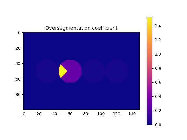
Briefly, the function computes the ratio between a characteristic lenght of the maximum contact area and a characteristic length of the particle. We can see that we can use a threshold of 0.5 to identify the particle that we need to fix. However, it is strongly recommended to select this threshold after a visual inspection (you can save the oversegmented label image, load it in Fiji,

and see how the threshold will affect the selection of the particles). This must be done since there is no unique value for this threshold, since it depends on the morphology of the grains, the morphology of the contacts (flat-flat contacts will have relative high overseg coefficients for example), and the mechanics of particles (deformable particles will increase their contact area, thus increasing their overseg coeff). With the list of target labels at hand, we can now run the function to fix the oversegmentation. Basically, the function merges the target particle with the one that generates the coefficient.

targetOver = numpy.where(overSegCoeff > 0.5)[0]
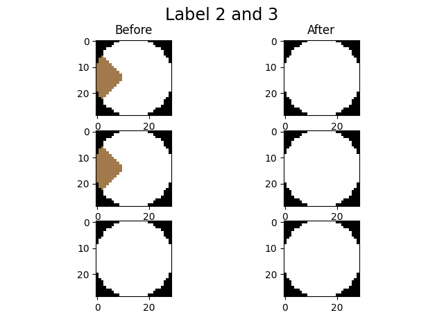
imLabel3 = spam.label.fixOversegmentation(imLabel2, targetOver, touchingLabels, imShowProgress=True, verbose=True)

|                                                             | ETA:  --:--:--
|##############################################################| ETA:  0:00:00
|##############################################################| Time: 0:00:00

We activated the imShowProgress key, so we can see (label by label) the result of the function. Let’s take a look at the current state of the label image

fig = plt.figure()
plt.subplot(1, 1, 1)
plt.gca().set_title("Label image")
plt.imshow(imLabel3[50, :, :], cmap=spam.label.randomCmap)
plt.show()

Important remarks

These functions are helpfull up to a point. It is strongly suggested to perform several iterations of detectOverSeg -> fixOverSeg -> detectUnderSeg -> fixUnderSeg. In order to obtain a “perfect”

label image, it is recommended to use Fiji to manually correct the labels that (for any reason) are not fixed by the functions.