
Note
Go to the end to download the full example code.
Expectation of global descriptors in 3D#
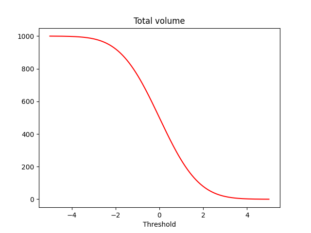
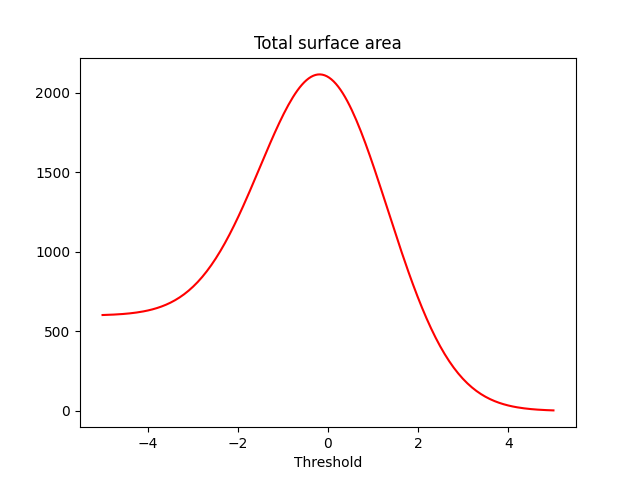
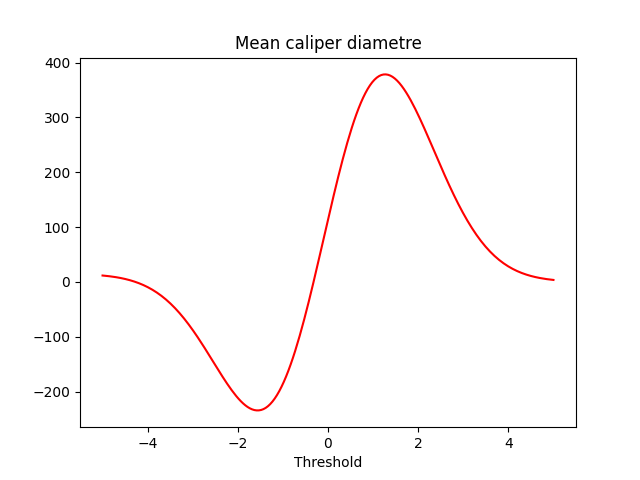
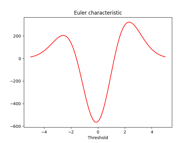
This example shows how to compute theoretical expectations of total volume (L3), surface area (L2), mean curvature measure (L1) and Euler characteristic (L0) of excursion sets as a function of the excursion’s threshold. Excrusions are define here as the subdomain of the domain where the Random Field is defined where the Random Field values are above a certain threshold.
Here the two measures are seen as function of the threshold value.
Monte Carlo results are confronted to the theory.
import spam.excursions
import spam.measurements
import matplotlib.pyplot as plt
import numpy
Compute the four theoretical expected measures#
The four measures of the excursion are computed and ploted for every thresholds
# spatial dimension
spatialDimension = 3
# the measure number 3
totalVolume = spam.excursions.expectedMesures(thresholds, 3, spatialDimension, std=std, lc=correlationLength, a=length)
# the measure number 2
totalSurface = 2.0 * spam.excursions.expectedMesures(thresholds, 2, spatialDimension, std=std, lc=correlationLength, a=length)
# the measure number 1
caliperDiameter = 0.5 * spam.excursions.expectedMesures(thresholds, 1, spatialDimension, std=std, lc=correlationLength, a=length)
# the measure number 0
eulerCharac = spam.excursions.expectedMesures(thresholds, 0, spatialDimension, std=std, lc=correlationLength, a=length)

plt.figure()
plt.xlabel("Threshold")
plt.title("Total volume")
plt.plot(thresholds, totalVolume, 'r')

plt.figure()
plt.xlabel("Threshold")
plt.title("Total surface area")
plt.plot(thresholds, totalSurface, 'r')

plt.figure()
plt.xlabel("Threshold")
plt.title("Mean caliper diametre")
plt.plot(thresholds, caliperDiameter, 'r')

plt.figure()
plt.xlabel("Threshold")
plt.title("Euler characteristic")
plt.plot(thresholds, eulerCharac, 'r')
[<matplotlib.lines.Line2D object at 0x7f584d183ee0>]
Generate 5 realisations of the correlated Random Field#
In order to compare the theoretical values to Monte Carlo results, first 5 realisations of a correlated Random Field are generated.
# number of realisations
nRea = 5
nNodes = 100

# define the covariance
covarianceParameters = {'var': variance, 'len_scale': correlationLength}

# generate realisations
realisations = spam.excursions.simulateRandomField(
    lengths=length,
    nNodes=nNodes,
    covarianceParameters=covarianceParameters,
    dim=spatialDimension,
    nRea=nRea)
Generating Field_0000... 32.43 seconds
Generating Field_0001... 32.35 seconds
Generating Field_0002... 32.56 seconds
Generating Field_0003... 32.47 seconds
Generating Field_0004... 32.49 seconds
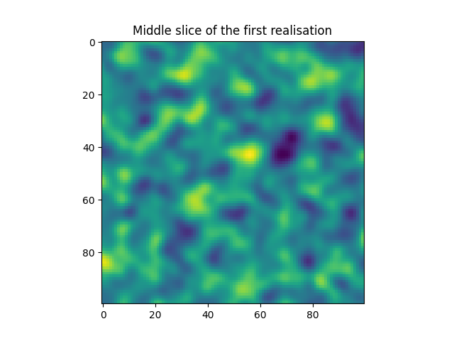
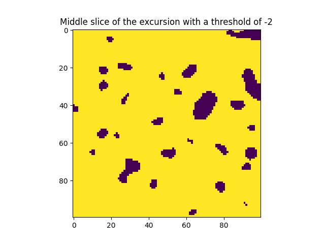
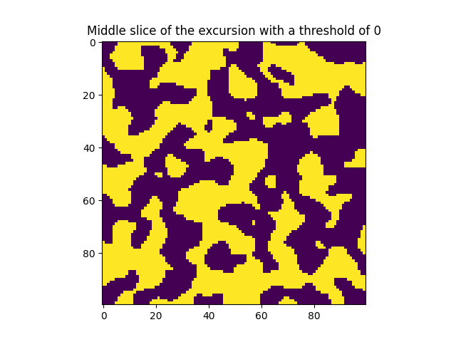
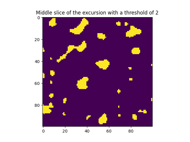
We now show, on the left, a slice a the first realisation and on the right the corresponding excrusion for 3 thresholds values: -2, 0 and 2 which corresponds to three different topologies.
plt.figure()
plt.title("Middle slice of the first realisation")
plt.imshow(realisations[0][int(nNodes / 2), :, :])

plt.figure()
plt.title("Middle slice of the excursion with a threshold of -2")
plt.imshow(realisations[0][int(nNodes / 2), :, :] > -2)

plt.figure()
plt.title("Middle slice of the excursion with a threshold of 0")
plt.imshow(realisations[0][int(nNodes / 2), :, :] > 0)

plt.figure()
plt.title("Middle slice of the excursion with a threshold of 2")
plt.imshow(realisations[0][int(nNodes / 2), :, :] > 2)
<matplotlib.image.AxesImage object at 0x7f5852631fc0>
Compute the four averaged measures (actually three)#
For every thresholds, three average measures (L0, L2 and L3) over all the realisations are compute and compared to the theoretical values.
# save average for every thresholds
totalVolumeMC = numpy.zeros_like(thresholdsMC)
totalSurfaceMC = numpy.zeros_like(thresholdsMC)
caliperDiameterMC = numpy.zeros_like(thresholdsMC)
eulerCharacMC = numpy.zeros_like(thresholdsMC)
# compute the aspect ratio
ar = length / float(nNodes)
# loop over the thresholds
for i, t in enumerate(thresholdsMC):
print(f"Threshold: {i + 1}/{len(thresholdsMC)}: {t:.2f}")
# loop over the realisations
for r in realisations:
totalVolumeMC[i] += spam.measurements.volume((r > t), aspectRatio=(ar, ar, ar)) / float(nRea)
totalSurfaceMC[i] += spam.measurements.surfaceArea(r, level=t, aspectRatio=(ar, ar, ar)) / float(nRea)
# commented because requires too much ressources
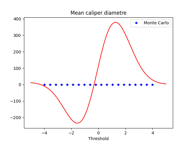
# caliperDiameterMC[i] += spam.measurements.totalCurvature(r, level=t, aspectRatio=(ar, ar, ar))/(float(nRea)*2.0*numpy.pi)
eulerCharacMC[i] += spam.measurements.eulerCharacteristic((r > t)) / float(nRea)
print(f"\t volume = {totalVolumeMC[i]:.2f} \t (err = {abs(totalVolume[i] - totalVolumeMC[i]) / abs(totalVolume[i]):.2f})")
print(f"\t surface = {totalSurfaceMC[i]:.2f} \t (err = {abs(totalSurface[i] - totalSurfaceMC[i]) / abs(totalSurface[i]):.2f})")
print(f"\t caliper = {caliperDiameterMC[i]:.2f} \t (err = {abs(caliperDiameter[i] - caliperDiameterMC[i]) / abs(caliperDiameter[i]):.2f})")
print(f"\t euler = {eulerCharacMC[i]:.2f} \t (err = {abs(eulerCharac[i] - eulerCharacMC[i]) / abs(eulerCharac[i]):.2f})")
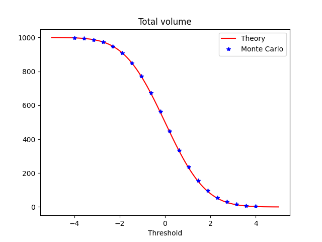
Threshold: 1/20: -4.00
volume = 997.67 (err = 0.00)
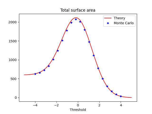
surface = 626.12 (err = 0.04)
caliper = 0.00 (err = 1.00)
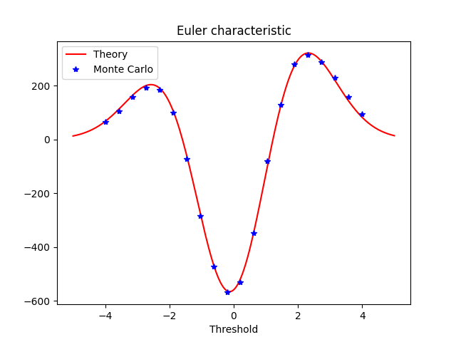
euler = 65.40 (err = 4.15)
Threshold: 2/20: -3.58
volume = 994.20 (err = 0.01)
surface = 661.17 (err = 0.10)
caliper = 0.00 (err = 1.00)
euler = 112.80 (err = 7.08)
Threshold: 3/20: -3.16
volume = 986.81 (err = 0.01)
surface = 728.03 (err = 0.20)
caliper = 0.00 (err = 1.00)
euler = 161.80 (err = 9.55)
Threshold: 4/20: -2.74
volume = 972.75 (err = 0.03)
surface = 840.56 (err = 0.39)
caliper = 0.00 (err = 1.00)
euler = 196.60 (err = 10.68)
Threshold: 5/20: -2.32
volume = 948.15 (err = 0.05)
surface = 1012.94 (err = 0.67)
caliper = 0.00 (err = 1.00)
euler = 185.60 (err = 9.06)
Threshold: 6/20: -1.89
volume = 908.12 (err = 0.09)
surface = 1247.56 (err = 1.06)
caliper = 0.00 (err = 1.00)
euler = 105.40 (err = 4.22)
Threshold: 7/20: -1.47
volume = 848.93 (err = 0.15)
surface = 1522.80 (err = 1.51)
caliper = 0.00 (err = 1.00)
euler = -64.80 (err = 3.93)
Threshold: 8/20: -1.05
volume = 768.46 (err = 0.23)
surface = 1792.46 (err = 1.95)
caliper = 0.00 (err = 1.00)
euler = -291.80 (err = 13.09)
Threshold: 9/20: -0.63
volume = 668.58 (err = 0.33)
surface = 1995.64 (err = 2.28)
caliper = 0.00 (err = 1.00)
euler = -476.80 (err = 19.10)
Threshold: 10/20: -0.21
volume = 554.91 (err = 0.44)
surface = 2074.72 (err = 2.40)
caliper = 0.00 (err = 1.00)
euler = -558.00 (err = 20.43)
Threshold: 11/20: 0.21
volume = 436.16 (err = 0.56)
surface = 1998.91 (err = 2.27)
caliper = 0.00 (err = 1.00)
euler = -515.60 (err = 17.50)
Threshold: 12/20: 0.63
volume = 322.66 (err = 0.68)
surface = 1774.16 (err = 1.90)
caliper = 0.00 (err = 1.00)
euler = -334.80 (err = 10.86)
Threshold: 13/20: 1.05
volume = 223.40 (err = 0.78)
surface = 1438.09 (err = 1.34)
caliper = 0.00 (err = 1.00)
euler = -61.00 (err = 2.65)
Threshold: 14/20: 1.47
volume = 144.95 (err = 0.85)
surface = 1070.29 (err = 0.74)
caliper = 0.00 (err = 1.00)
euler = 163.40 (err = 3.09)
Threshold: 15/20: 1.89
volume = 87.71 (err = 0.91)
surface = 732.31 (err = 0.19)
caliper = 0.00 (err = 1.00)
euler = 285.40 (err = 5.60)
Threshold: 16/20: 2.32
volume = 49.01 (err = 0.95)
surface = 457.10 (err = 0.26)
caliper = 0.00 (err = 1.00)
euler = 319.20 (err = 5.83)
Threshold: 17/20: 2.74
volume = 25.20 (err = 0.97)
surface = 260.93 (err = 0.58)
caliper = 0.00 (err = 1.00)
euler = 290.60 (err = 4.76)
Threshold: 18/20: 3.16
volume = 11.92 (err = 0.99)
surface = 134.00 (err = 0.79)
caliper = 0.00 (err = 1.00)
euler = 211.40 (err = 2.89)
Threshold: 19/20: 3.58
volume = 5.15 (err = 0.99)
surface = 62.25 (err = 0.90)
caliper = 0.00 (err = 1.00)
euler = 138.80 (err = 1.37)
Threshold: 20/20: 4.00
volume = 2.01 (err = 1.00)
surface = 26.01 (err = 0.96)
caliper = 0.00 (err = 1.00)
euler = 74.40 (err = 0.19)
We can now plot the theory and Monte Carlo measures over the thresholds
# plot volume
plt.figure()
plt.xlabel("Threshold")
plt.title("Total volume")
plt.plot(thresholds, totalVolume, 'r', label='Theory')
plt.plot(thresholdsMC, totalVolumeMC, '*b', label='Monte Carlo')
plt.legend()

# plot surface
plt.figure()
plt.xlabel("Threshold")
plt.title("Total surface area")
plt.plot(thresholds, totalSurface, 'r', label='Theory')
plt.plot(thresholdsMC, totalSurfaceMC, '*b', label='Monte Carlo')
plt.legend()

# plot caliper diametre
plt.figure()
plt.plot(thresholds, caliperDiameter, 'r')
plt.plot(thresholdsMC, caliperDiameterMC, '*b', label='Monte Carlo')
plt.xlabel("Threshold")
plt.title("Mean caliper diametre")
plt.legend()

# plot Euler characteristic
plt.figure()
plt.xlabel("Threshold")
plt.title("Euler characteristic")
plt.plot(thresholds, eulerCharac, 'r', label='Theory')
plt.plot(thresholdsMC, eulerCharacMC, '*b', label='Monte Carlo')
plt.legend()
plt.show()
Total running time of the script: (2 minutes 57.385 seconds)