
Tutorial: Contacts calculation#
Objectives of this tutorial#
This tutorial follows the lines of [Wiebicke2019] which provides code along the lines of what follows. The objective here is the characterisation of contacts between particles in a granular material. The first question will be the detection of a contact between two grains, which has been carefully studied in [Wiebicke2017], thereafter we will try to measure its orientation. In this tutorial we will start from a ground truth: it is a sythnetic assembly of spheres coming from a Discrete Element simulation with [Woo]. The state which is studied is one of isotropic compression – the system is in mechanical equilibirum (i.e., there are a reasonable number of contacts between particles).
Generating synthetic image#
Using the example given here (with a pixel size of 15µm/px, blur of 0.8 and noise of 0.03) Kalisphera sphere assembly generation we generate a synthetic image with a known amount of blur and noise.
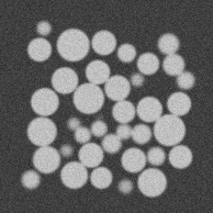
It’s important to note however that we know the ground truth from the original data, i.e., which particles are in contact, and what the contact orientation is (it is the in the direction of the vector linking sphere centres).
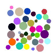
Clearly a first step is to label the grains as per Tutorial: Label Toolkit. Since the sythnetic data has pores = 0.25 and solid = 0.75 we know that the threshold to classify voxels more than 50% occupied with solids is >0.5:
# ...following from kalisphera example
import spam.label
lab = spam.label.watershed(Box>0.5)
which gives:
Detecting contacts#
From this labelled image, a first naive approach is just to see which labelled voxels are touching voxels of another label:
contactVolume, Z, contactsTable, contactingLabels = spam.label.labelledContacts(lab)
import matplotlib.pyplot as plt
plt.hist(Z)
plt.xlabel("Number of contacts per particle")
plt.ylabel("Count")
plt.show()
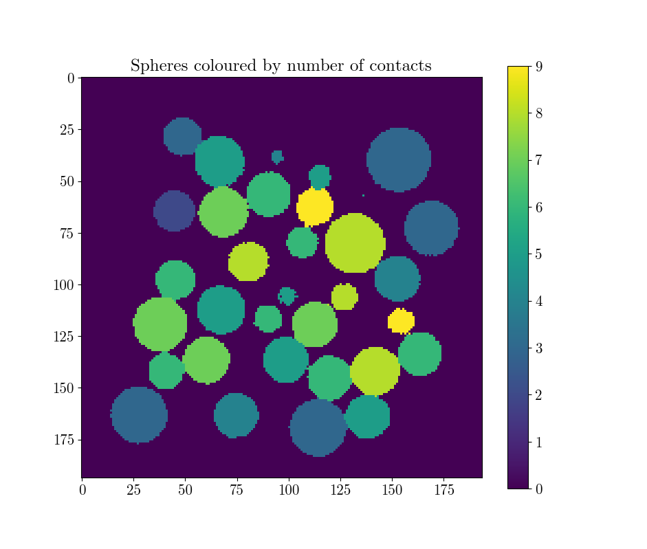
plt.imshow(spam.label.convertLabelToFloat(lab, Z)[Box.shape[0]//2])
plt.title("Spheres coloured by number of contacts")
plt.colorbar()
plt.show()
This yields the following distribution of coordination number (i.e., the number of contacts per particle), and its distribution per-sphere:
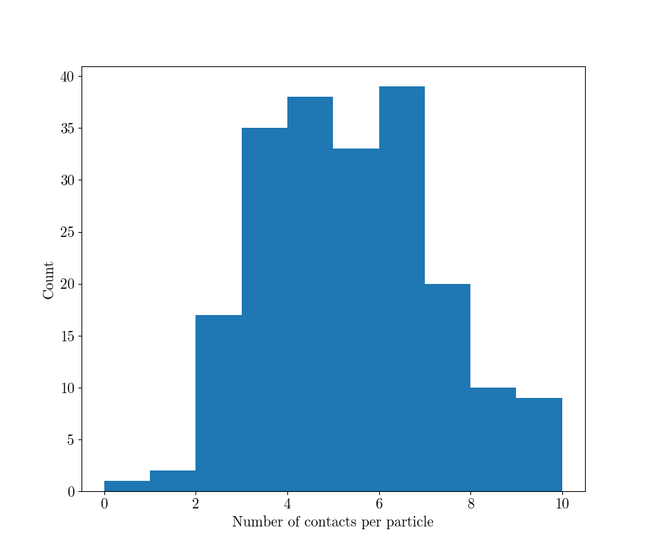
As clearly demonstrated in [Wiebicke2017] this is a systematic one-sided overestimation of true number of contacts, since close contacts are over-detected according to an over-detection distance, even without blur and noise. spam.label has implemented the improvement technique suggested in that paper, which will use a local threshold to reduce this over-detection. The value of this threshold has been taken directly from the paper, but needs to be calibrated carefully before use:
localThreshold = 180/255.0

contactingLabelsRefined = spam.label.localDetectionAssembly(lab, Box, contactingLabels, localThreshold)
uniqueLabels, uniqueCounts = numpy.unique(contactingLabelsRefined, return_counts=True)
Zrefined = numpy.zeros(uniqueLabels.max()+1)
for l, c in zip(uniqueLabels, uniqueCounts):
    Zrefined[l] = c
If load and compare to the contacts in original DEM data (these are given from the DEM collider):
contactListDEM, _ = spam.datasets.loadDEMtouchingGrainsAndBranchVector()
uniqueLabels, uniqueCounts = numpy.unique(contactListDEM, return_counts=True)
Zdem = numpy.zeros(int(uniqueLabels.max())+1)
for l, c in zip(uniqueLabels, uniqueCounts):
    Zdem[l] = c

# Plot three distributions of coordination number together to compare
plt.hist(Z, histtype='step', label="Naive Coordination Number")
plt.hist(Zrefined, histtype='step', label="Improved Coordination Number")
plt.hist(Zdem, histtype='step', label="DEM (reference) Coordination Number")
plt.xlabel("Number of contacts per particle")
plt.ylabel("Count")
plt.legend()
plt.show()
Which shows how much of an overestimation the naive method with the expected threshold value is, and the significant improvement given with a higher threshold.
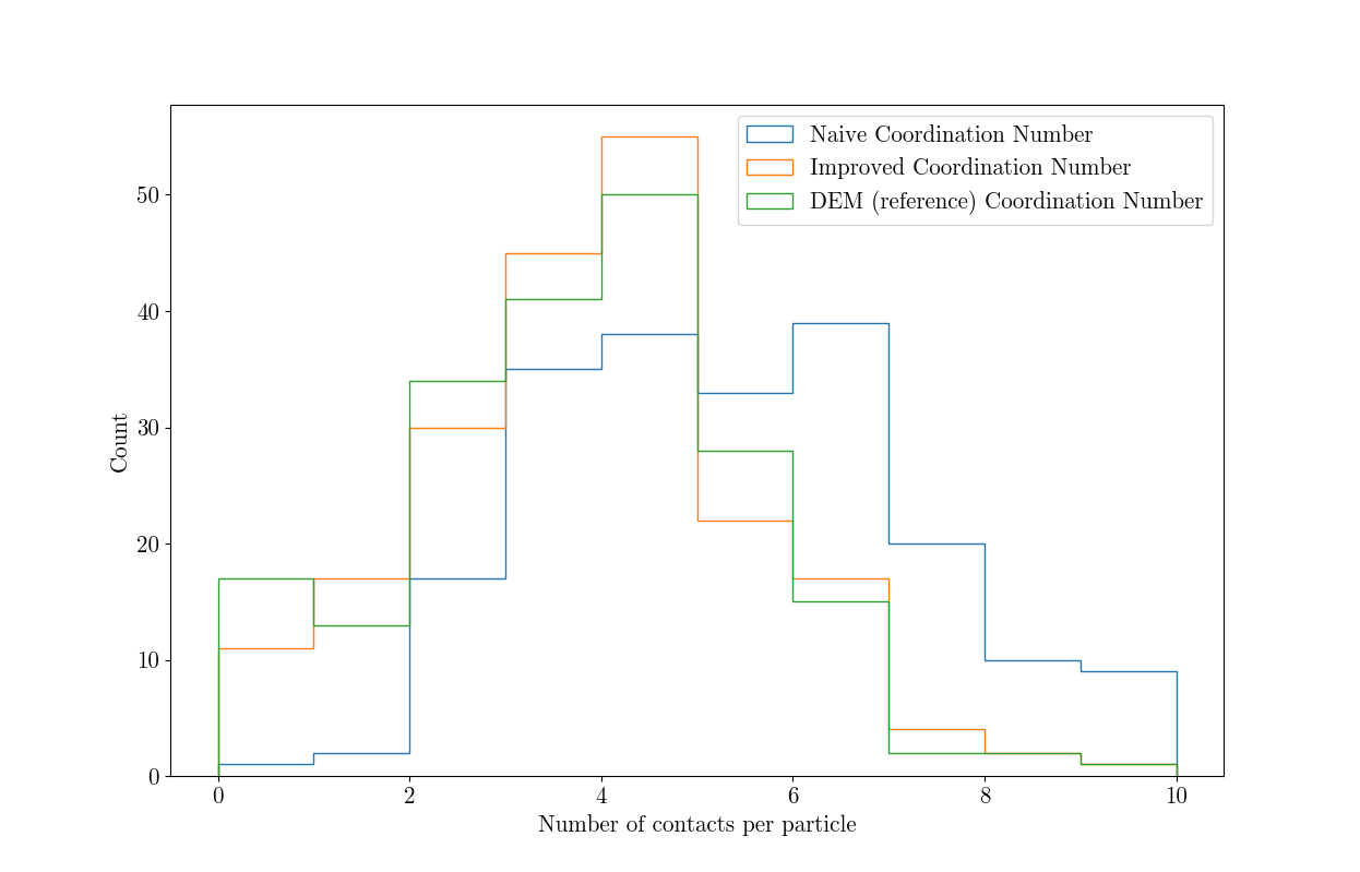
The mean coordination number is also significantly improved:
print("Mean Coordination Original:        ", Z.sum()/lab.max())
print("Mean Coordination Refined:         ", Zrefined.sum()/lab.max())
print("Mean Coordination DEM (reference): ", Zdem.sum()/lab.max())
Mean Coordination Original: 4.89
Mean Coordination Refined: 3.43
Mean Coordination DEM (reference): 3.32
…A huge improvement.
Measuring Orientations#
Once we are happy with the identified contacts, we can start calculating their orientations. Currently, there are two different approaches implemented in spam. The first determines the orientation based on the labelled image and is therefore called watershed=”ITK”. The second technique segments each pair of contacting grains additionally using the random walker, which allows a far more accurate determination of the contact orientation. It is called with watershed=”RW”. We strongly recommend the random walker segmentation, although it is more time consuming. You can assign NumberOfThreads to distribute the calculation to multiple nodes. The orientations can be calculated by:
contactOrientations = spam.label.contactOrientationsAssembly(lab, Box, contactingLabelsRefined, watershed="RW", nProcesses=2)
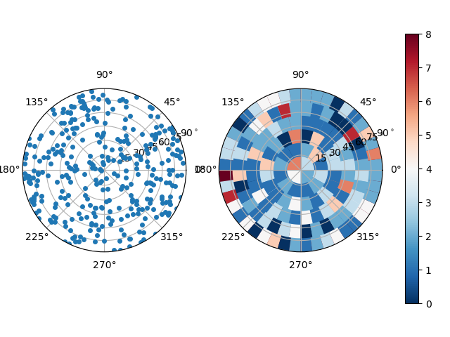
Note that the orientations are saved in (z,y,x) order as given in the Module Index. The orientations can then be plotted, using for example the orientation plotter implemented in spam.:
import spam.plotting
spam.plotting.plotOrientations(contactOrientations[0:,2:5], plot="both", numberOfRings=6)
Which results in a plot of the individual orientations as points and a binned version which is usefull when thousands of orientations are to be plotted.
As done for the coordination number, we can also compare the orientations to the reference. Remind that the reference is the DEM simulation, that was used to create this assembly of spheres. It can be loaded from the examples:
_, referenceOrientations = spam.datasets.loadDEMtouchingGrainsAndBranchVector()
Here, we compare the orientations that are calculated from the images using either the ITK watershed or the random walker with the reference orientations from the DEM simulation.
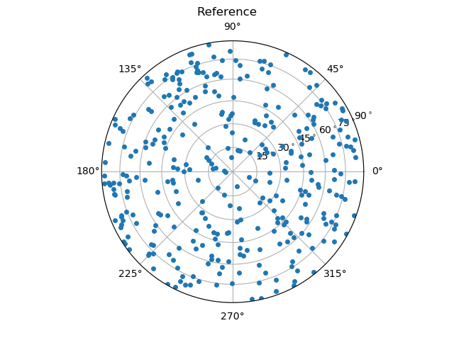
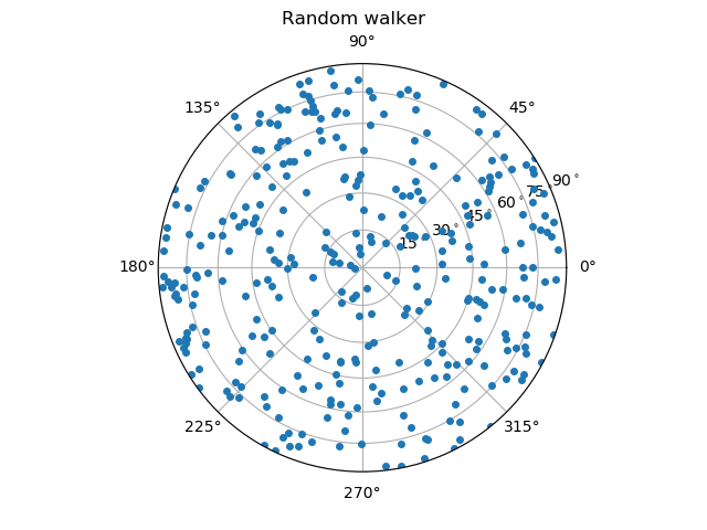
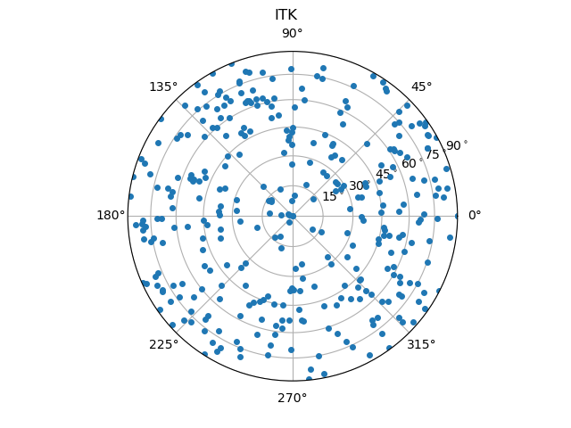
From these images, one can already guess that the random walker approach produces more accurate results. A more thorough metrological analysis is presented in [Wiebicke2019].
Note
Note that the determination of orientation gets substantially more complex and error-prone for irregularly shaped grains. If the calculation runs into problems, it will output a zero vector for the contact pair. These vectors have to be deleted (or neglected) from the orientations in order to work on the data set. As the orientations are calculated by performing a principal component analysis the number of data points corresponds to the quality of the fit. This number is given as the last entry (column) of the contactOrientationsAssembly(). It is recommended to exclude orientations with very few (I usually exclude at about less than 10 for Hostun Sand at 15 micro meter) and very many of these data points (oversegmentation). These values depend on the spatial resolution of the tomographies.
Capturing fabric#
In order to capture the fabric, we need to treat all the individual orientations statistically. The most common way to do so, is to employ a second order fabric tensor. We follow the definitions from [Kanatani1984]. The fabric tensor, it’s deviatoric part and a scalar anisotropy factor can be computed by:
N, F, a = ltk.fabricTensor(contactOrientations[:,2:5])
The fabric tensor in this example would then read:
[[ 0.318  0.007  0.006]
[ 0.007  0.319 -0.009]
[ 0.006 -0.009  0.363]]
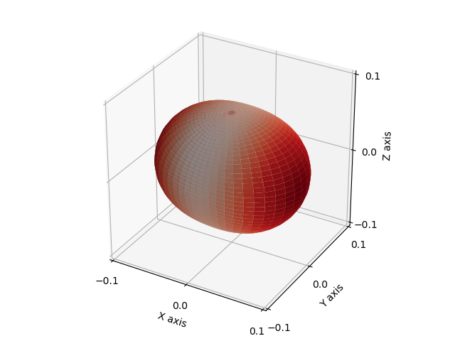
In order to visualise the fabric, we can use the distribution density function of the deviatoric part of the fabric tensor as described in [Kanatani1984]:
spam.plotting.orientationPlotter.distributionDensity(F)
This surface is additionally colored by its radius in order to simplify observing preferential orientations. In our case, the preferential orientation of the tensor is colored with red.
References#
Wiebicke, M., Andò, E., Šmilauer, V., Herle, I., & Viggiani, G. (2019). A benchmark strategy for the experimental measurement of contact fabric. Granular Matter, 21(3), 54. https://doi.org/10.1007/s10035-019-0902-x
Wiebicke, M., Andò, E., Herle, I. & Viggiani, G. (2017). On the metrology of interparticle contacts in sand from x-ray tomography images. Measurement Science and Technology, 28 124007. https://doi.org/10.1088/1361-6501/aa8dbf
Šmilauer, V. (2016). Woo documentation. https://www.woodem.org/index.html
Kanatani, K.-I. (1984) Distribution of directional data and fabric tensors. International Journal of Engineering Science, 22(2):149 – 164. https://doi.org/10.1016/0020-7225(84)90090-9